Skoči na glavni sadržaj

Izvorni znanstveni članak

https://doi.org/10.7906/indecs.20.5.8

On Employing of Extended Characteristic Surface Model for Forecasting of Demand in Tourism

Janusz Opiła orcid id orcid.org/0000-0003-1179-1920 ; AGH University of Science and Technology Cracow, Poland


Puni tekst: engleski pdf 2.083 Kb

str. 621-639

preuzimanja: 88

citiraj

Preuzmi JATS datoteku


Sažetak

Extended Characteristic Surface Model is a theoretical tool of general application designed for computing coefficients in Monte Carlo stochastic simulations in particular in multi equation stochastic econometric models. Econometric models are most often used for economic analysis of large enterprises as well as national economies but rarely for analysis of small entities. The reason is that the costs of building and testing such large-scale models are very high. However, the hereby presented Extended Characteristic Surface Model delivers a not-so-expensive, rather intuitive, and flexible method eligible for consumer sentiment analysis and forecasting as well as for "what-if" inferring suitable for entities of all sizes. In particular, it allows for analysis of demand variation resulting from messages concerning competing merchandise. The article is focused on the application of the Extended Characteristic Surface Model for the evaluation of sentiment and forecast of demand in tourism. In the work extended characteristic surface method is explained in thorough detail, furthermore, the influence of factors such as demographic structure, prices, or market size on financial outcomes is analysed on the example of a small touristic entity.

Ključne riječi

forecasting; sentiment; tourism; visualization; machine learning

Hrčak ID:

284157

URI

https://hrcak.srce.hr/284157

Datum izdavanja:

31.10.2022.

Posjeta: 403 *


INTRODUCTION

For evaluation of business enterprises, complex multi-parameter econometric models are build up. As it is well known that tiny variations of input data may induce large changes on output, econometric models are employed for the analysis of the sensitivity of an entity to viable internal and external conditions often changing very abruptly. As probing input data combinations is impossible partly due to obvious danger of irreparable damages to the entity, experimenting on the mathematical model is safe and allows for reliable what-if analysis and forecasting. Econometric models are sets of mutually conjugate equations based on time series of economic categories often delayed. Such models consist generally of two elements: time series of econometric categories and set of coefficients relating them. Thus accuracy of coefficients is crucial for reliability of the model. Common methods of evaluation of coefficients are e.g. ARMA (Autoregressive Moving Average), ARIMA (Autoregressive Integrated Moving Average), ARMAX (Auto Regressive Integrated Moving Average with eXogeneous Input) or regression-based methods. Unfortunately, this gives point estimates only while due to imminent inaccuracy of learning datasets they are rather interval estimates. There are generally two attempts to overcome this limitation – Monte Carlo simulations and fuzzy number or interval arithmetic – both have pros and cons. Fuzzy number methods despite intense research and development still suffer problems concerning computation complexity as well as convergence1. However, the solution may be obtained in a single computation pass2. Oppositely Monte Carlo based methods are presently very well explored. However, in order to produce reliable results, they require multiple repetitions of every simulation pass and subsequent statistical analysis. Another problem is the need to use long and uncorrelated series of random numbers, however present day pseudorandom number generators, like Mersenne Twister3, Matsumoto4, allows to overcome this limitation. The direct bonus of this procedure is obtaining empirical probability distribution estimate of output data. Furthermore, due to enormous computation power of contemporary computers, considerable computation complexity of Monte Carlo based methods is no more the problem5. One of the problems of MC based methods is often complex and hard to assess structure and hierarchy of conditional decisions. In the article, hypothesis is verified that Monte Carlo based Characteristic Surface Model is useful for modelling of economic output of a single small touristic entity in the era of pandemic. Alongside numerical efficiency of the Model, ability to recreate typical scenarios will be investigated as well as ability of assessment of risk level and of estimation of fluctuations level. For the case study, Croatian touristic industry was selected due to its specificity including strong influence on the State economy. The Methodology section consists of 6 subsections. In the first specificity of tourism in Croatia is analysed. In the second one, Characteristic Surface Method, extended characteristic surface model (eCSM) is introduced as an efficient tool for determination of stochastic coefficients in econometric models. Accordingly, relevant terminology is explained. In the next section, Design of the Numerical Experiments, experimental setup is presented and explained. In the fourth section, econometric model of hypothetic private, small touristic entity is presented as a base for calculations presented in the next section. Characteristics of layers adopted in this exemplary case is presented in Layers Data subsection. In the last subsection computer program written as test tool for the case study has been described, as well as other software utilized. In the next section, Results, attempt is made to perform numerical modelling of evolution of consumer sentiment using characteristic surface method on the example of tourism industry in the era of SARS-Cov-2 pandemic. In particular, applicability of estimation of influence of input data, (e.g. population structure) on model output values is analysed. Computational results for eight different scenarios are presented; two examples display influence of discounts on final profit of the entity. Next two sections are devoted to discussion of results and presentation of final conclusions.

METHODOLOGY

Specificity of Tourism in Croatia For the case study, tourism in Croatia has been chosen due to its remarkable specificity. Economics of Croatia, as well as more than 40 other countries, depends heavily on tourism. According to some authors, share of tourism in overall economy for 2017 was about 19,6 %, which is almost one third of the whole services sector ‒ 70,1 %6,7 compared to industrial output at 26,2 % and agriculture 3,6 %. Other sources give even higher figures up to 25 % in year 2019 and 383 400 jobs (9,3 % of population) involved in the tourism industry8. Different figures may result from taking into account real contribution to Gross Domestic Product (GDP) accounted for 15.2 billion of US$9, while the other may include revenues (13 billion US$ in year 2019) of touristic industry only8. Due to analysis of Orsini and Ostojić10, Croatia has the highest share of tourist revenues in GDP among countries like Cyprus, Greece, Malta, Italy, and Spain. This makes Croatian economy very sensitive to even minor fluctuations. At real GDP PPP accounting $116,34 in 20197 Croatia was 85th country in the world, however taking into account GDP per capita ($28 602) was even higher ‒ 72nd which means substantial progress if compared to year 20177,11. After a collapse initiated in 2008 by world financial crisis Croatia started recovery in late 2014 which culminated in 2019 at GDP growth rate at 2,9 %, declining public debt (to 73,2 % of GDP) (The World Bank12) and notable reduction of unemployment rate to below 7 % from 15 % in 2015 (7). It was speculated that due to SARS-Cov-2 outbreak, GDP may shrink by more than 8,1 %. Unemployment rate was estimated at 7,5 % in 2020 Q311 while previous estimates were even higher at 9 %. While governmental emergency package (Croatia Week13) may help reducing the economy downturn, it was forecasted, that it would increase budget deficit and substantial rise of public debt even up to 84 % GDP by the end of 2020. Moreover, a fiscal deficit may set a record rising close to 7 % of GDP. It was expected that economy would rebound in the second half of 2020 (The World Bank,12) but no conclusive figures are available yet. It is expected that pre-epidemic levels may be reached no sooner than in 202214. Decline in number of overnights in 2020 was not distributed evenly. For example, Rab island, claimed as “Covid free zone” noticed only minor decrease of number of tourists15. This stresses up role of FUD (fear, uncertainty and doubt) in planning or abandoning holiday travel plans. Characteristics of tourism in Croatia changed abruptly in 1995. Up to 1995 the shares of domestic and foreign tourists were comparable, however thereafter share of domestic tourists remained on war time level, while number of foreign tourists rapidly rebounded to a record number of 21 million in 2019 (5 % increase vs. 201816-18). This has changed in 2020, as in March only drop of 75 % in number of tourists was recorded year to year19. Figures for the April were even more severe reaching 99,8 % drop19. However preliminary data showed that in a whole year reduction of overnights was lesser than expected, at 54,0 million versus 91,24 million in year 2019 (59,2 %)18,20. Accommodation structure is one of the most interesting factors of Croatian tourists industry17,18. While number of beds in hotels and camping sites barely grows or even decreases, number of beds in private accommodation entities more than tripled compared to year 1995 (Figure 1). Not only does it make Croatian tourism unique, but also has important social and economic consequences e.g., by helping reducing jobless rate (very high among youth, 17,8 % in 201921) as many facilities are operated by families. Another fast-growing tourism sector is nautical tourism18; p.33, which stayed unexpectedly strong amid epidemic in year 202022. This may be attributed to adventurous nature of sailors. Structure of private accommodation in Croatia is moderately diversified. Based on data from rental agencies, offered entities range from small, one or two apartments (rooms or studios) facilities up to luxury micro hotels for say ten families. What makes them distinct from regular hotels is management ‒ private accommodation is by rule governed by a single family or even one person only. Average number of overnights per arrival depends on the month. In the summer, it approximates to six days/one week (July, August), 5 days in June and September and less than three days in the rest of the year. This is probably caused by policy of owners of private accommodations and camps who restrict reservations to the whole week in high season and lift that limitation in other months17,18. Furthermore, number of overnights vary during the year and peaks in July/August far more than in other countries10. Strong seasonality is another weakness of tourist industry.

Figure 1. Number of beds depending on accommodation type

18

indecs-20-621-g1.png
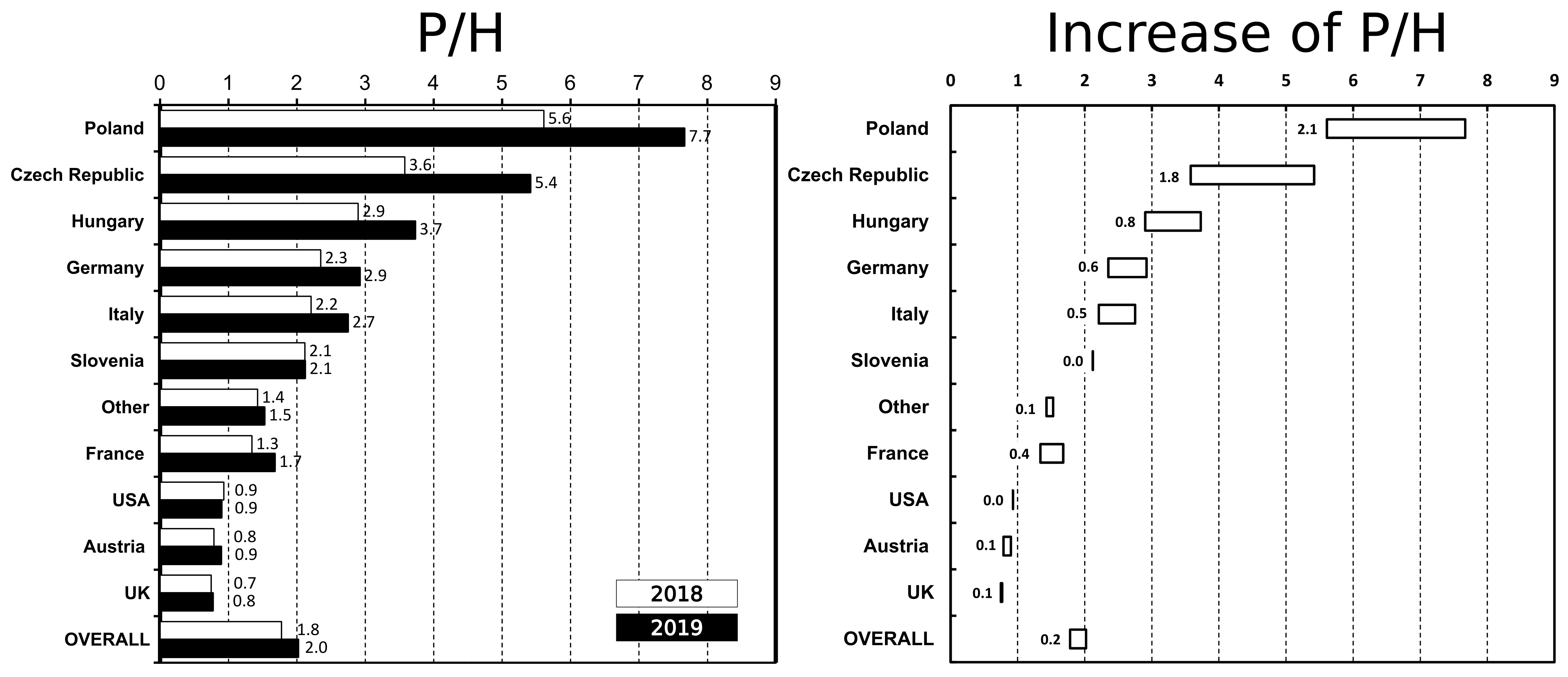
Average number of overnights per arrival depends on country of origin too. While tourists from Germany, Czech Republic and Poland arrive to Croatia for one week on average (7,2, 6,8 and 6,5 respectively), the ones from Austria, Slovenia, Hungary, UK and Italy stay for approximately 5 days18. Visits from other countries are shorter than four days. According to governmental data in 2020 only number of overnights generated by tourists from Poland was substantially higher than in 201923, peaking at 12,4 % of all bed nights a bit less than Slovenes tourists (13,5 %) but ahead of Czechs (9,2 %) and Austrians (6 %) while Germans retained first place with 33,3 % of all overnight stays24. What is intriguing is that the choice of accommodation type strongly depends on the country of origin. It may be best presented as dependency of proportion of number of overnights in private accommodation and the number of overnights in hotels, on the country of origin – P/H. Based on data from y.201918, four different groups may be spotted (Figure 2). The first one contains only one country – Poland (P/H = 7,67). The second group consists of Czech Republic, Hungary, Germany, Italy and Slovenia (2,1 < P/H > 5,42). To the third one belongs France and “other countries” (1,5 < P/H > 1,7). The last one consists of USA, Austria and UK (P/H < 1.0). While sentiment of Polish tourists toward private accommodation may be attributed to more affordable prices or just preferred form of vacationing, the difference between Austria and Germany is more difficult to understand. Both countries are comparably wealthy and are in similar distance from Croatia with Austria being obviously nearer. This puzzle should be explained in separate research. There is one more thing to note, namely rapid grow of P/H factor for some countries like Poland or Czech Republic with stagnation for others like Slovenia, UK or USA (Figure 2, right). P/H factor lesser than one, spotted for travellers from USA, Canada or UK may be attributed to luggage limitations imposed by airlines. This makes hotels the first choice for accommodation. However, this does not explain low value of P/H factor for Austria i.e. 0,9 (0,7 in 2018), as Croatia is easily accessible by car and there are no serious luggage limitations. Larger figures for private accommodation may result also from that increase of number of hotel beds requires more investments, thus owners of private accommodations tune to market requirements faster. Analysis of available offers suggests that typical price per week/per arrival ranges from 400 up to 600 €, however prices over 1000 € per week are not uncommon. It should be stressed that as the euro is widely accepted (and often expected) in all payments (services, restaurants, tolls and goods) it became the second currency of Croatia, even prior to official access to Eurozone, expected as soon as in year 2022 as Croatia currently participates in the ERM II since July 10th 202025.
Figure 2. Proportion of overnights in private accommodations to hotel overnights (P/H) vs. country of origin
indecs-20-621-g2.png
Comparison of P/H factor for year 2019 vs. year 2018 (left) and illustration of increment (right). White fill means increment, black decrease or no change18. Summarizing, majority of tourists in Croatia is from abroad, spent one week per arrival most likely in private accommodation; all payments may be done in the euro. Numerical experiments presented in the next chapter are based mainly on these conclusions. Details of Characteristic Surface Method The method is being developed for some years. In the course of time some important and promising results have been obtained and presented in national journals, selected papers26,28. However, method with latest improvements has not been presented yet in details at the international forum not including more or less descriptive presentation29-31. Thus the article is devoted to detailed description of both theoretical background of the method and crucial details of implementation. The model is built upon specific to the model notions and assumptions defined as follows. Abstract population P consists from I “individuals” ‒ exemplary it may be group of tourists, but individuals of other kind may be regarded too, namely migrating birds or animal species choosing between two habitats. Many other kinds of “individuals”, including elementary particles or molecules may be the subject of the model. Individuals are making personal “decisions” choosing one of at least two options ‒ M options in general. Although model allows for values of M > 2, employing M = 2 should be sufficient for majority of typical scenarios. In particular M = 2 allows to model the financial outcome of economical entity under consideration (one option) versus its competitors (second option). However, increasing number of options beyond 2 may sometimes be necessary. So, for the sake of simplicity, M = 2 will be assumed in this article. For each individual every option has an individually attributable “attractivity” Ai, i = 1, ..., M. Each individual selects one option according to all values of Ai, exact reason for selecting given option Ai is intentionally assumed unknown, irrelevant and it does not matter if it was selected consciously and by reason or spontaneously, however it is assumed that sentiment towards different options remains fairly constant over time. Act of decision may be modelled using “criterion function” K(A1, A2, …, AM) which evaluates to whole numbers 1, 2, …, M depicting which option has been selected. In order to make model computable it is further assumed that a transfer function f(A) exists converting elusive attractivity A into real number a: a = f(A). Finally criterion function is defined as m = K(f(A1), f(A2), …, f(AM)) = K(a1, a2, …, aM), where m = 1,2, …, M is the number of the option selected. Probability of drawing of individual with a set of attractiveness A = {A1, A2, …, AM} is governed by function CS( ) of M variables: z = CS(a1, a2, …, aM), which may be interpreted as multidimensional probability density function, PDF in short. This is the most important part of the model actually. It is assumed that the shape of the function is rather constant for the given population over longer times or evolution of the function CS(a1, a2, …, aM) is predictable by direct computation, forecast or modelling. Thus, because the function CS(a1, a2, …, aM) is characteristic to the given population over some time interval, it has been named Characteristic Surface and the whole model, Characteristic Surface Model (CSM). While early implementations employed static characteristic surface, the latter probe dynamic surfaces, i.e. changing over time. In order to model the evolution of the characteristic surface over time and due to variety of signals (signal ‒ a prominent event influencing behaviour of the population, e.g. epidemic) or conditions (i.e. set of parameters e.g. interests rates or mortgage loans rates), a variety of methods may be used. For example, the following may be mentioned: forecasting or control models, e.g. ARIMA (autoregressive integrated moving average), least squares based models GLM (General Linear Models), machine learning (ML) models, artificial intelligence (AI) trained models or last but not the least – formula based layer models. The last one is very useful for performing numerical experiments while probing theoretical background of the model. “Layer” is defined as a subset of all individuals of the population, similarly reacting to signals. Thus splitting the whole population into layers allows for individual modelling of the evolution of every single layer independently from others and as a result, modelling evolution of the complete characteristic surface. As every layer has its own shape function CS(a1, a2, …, aM), each one may be modelled independently from others. One may be defined by equation, the other by empirical PDF, and another by AI/ML model. Furthermore, while one layer evolves, the other may remain static. In that way the model allows for testing many diverse scenarios. In the article equation-based layers were used. Author found the use of time dependent correlated bivariate Gauss probability density distribution function G(μ1, σ1, μ2, σ2, ρ, t) as particularly useful, where μ1, μ2 are means, σ1, σ2 standard deviations, ρ correlation coefficient and ‘t’ indicates time dependency. In original implementation the domain of numeric attractiveness ai = f(Ai) was restricted to the unit square what was causing some troubleshoots. Current, enhanced implementation lifts this limitation so time evolution of CS may be modelled in a more consistent and logical way. Another possible enhancement is introduction of criterion function K dependent on previous decisions of selected individual, thus allowing introduction of personal experience into the model. The presented model does not provide procedure of evaluation of CS. Thus, variety of methods may be applied: query, theory of the subject, historical data, Big Data analysis, Machine Learning/Artificial Intelligence and A/B testing method [32 (known also as bucket or split run testing) or just formula ‒ whatever suits the best. Summarizing, the Characteristic Surface Model may be denoted as a set CSM consisting of Characteristic Surface CS, attractivity A and criterion function K: CSM = {CS, A, K}. Obviously, CSM is the function of the number of options M, number of layers L and time t. It is assumed that in the following analysis M = 2, there are three layers and one of them evolves with time. In order to emphasize the difference between static and dynamic formulations time dependent variant of the model was named “enhanced” thus finally acronym eCSM is used. Design of the Numerical Experiments In order to test and illustrate pros, cons and caveats of the model, hypothetical tiny tourists entity located in small destination has been selected. This is motivated by following assumptions and goals: • small entities are more sensitive to fluctuations of incomes and expenditures than bigger, • it is far more difficult to simulate small-scale entity than large-scale as fluctuations rapidly rise for small number of individuals/tourists, • as the number of small tourist entities is currently very big and still grows, it is important to test the tool for analysis of what-if scenarios for them. Econometric model and assumed data In the article, multi-equation stochastic econometric model of the agritourism farm, developed and tested in the past27,28 was adequately adopted and enhanced. Due to the exploratory nature of this research, some simplifications were accepted. The subject of the model is now a small touristic entity located in a small touristic destination (e.g., Soline, Šilo, Lumbarda, Postira). Host offers 6 apartments on weekly basis and earns flat price over whole season 20 weeks long, beginning June 1st. There is no problem with implementing a more complex scenario but this is far beyond the scope of the article. Weekly cost of the facility consists of constant part (instalments, local taxes, etc.) and variable costs depending on the number of flats rented (e.g., tourist tax, water, energy). Fixed costs per week are of course case-dependent. However, they may be deduced from yearly costs recalculated per one week in the season. Although according to official statements only about 8 % of loans indexed to CHF were taken for seaside rental houses33, such a case is taken into account in this experiment. According to the analysis performed by Tepuš34, the average monthly house instalments before 2005 were estimated at € 654. Another, though underrated, element of the private entity’s fixed costs are living costs of the owner and his family, spread over whole year. Therefore, the value of the fixed costs during the period considered was roughly assumed at EUR 1000 per week for the whole entity, keeping in mind that this cost component is strongly case dependent. Although not very high, model takes into account cost connected with not-rented apartments. No taxes explicitly are taken into account as local and other taxes are included implicitly in fixed and variable costs. It was assumed that whole population might be split into three distinct layers, represented by bivariate correlated Gaussian distribution every. For the testing purposes, basically two were assumed static while the third one was migrating (change of μ1 and μ2) and changing its dispersion parameters (σ1 and σ2), while keeping correlation coefficient p constant. Evolution patterns varied with the experiment. Summary of parameters of Model are presented in the Table 1. Other extended cases are explicitly described in the Results section and in the Table 2.

Table 1. Definition of the Stochastic Econometric Model.
VariableFormula, value or range assumedComment
‘t’0…20Index - week number
IR3000Initial financial resources in €
NR100Number of repetitions
N6Number of apartments for rent, constant
ND100Number of apartments for rent in destination, constant
pt420 € (315€, 360€)Basic price per week ‘t’and variations, assumed constant
Ft1000 €Fixed costs at period ‘t’, estimated,
DTot90, 135 or 200Total demand for the destination. Assumed constant.
CF,t10 €Cost of “free” apartment at time ‘t’
CU, t25 €Unit cost per apartment rented at time ‘t’
DtDt = D(t, …)Demand in period ‘t’, depends on many factors
NS, tNS, t = min(Dt , N)Number of rented apartments in period ‘t’, NS.t≤N
CtCt = Ft+NS, t CU, t + (N – NS, t)CF, tTotal cost of unit at week ‘t’; variable
ItIt = pt NS,tIncomes for week ‘t’
PtPt = It CtProfit per week ‘t’
PC,tPC,t = Pt + PC,t-1Cumulated profit, PC,0 = IR.

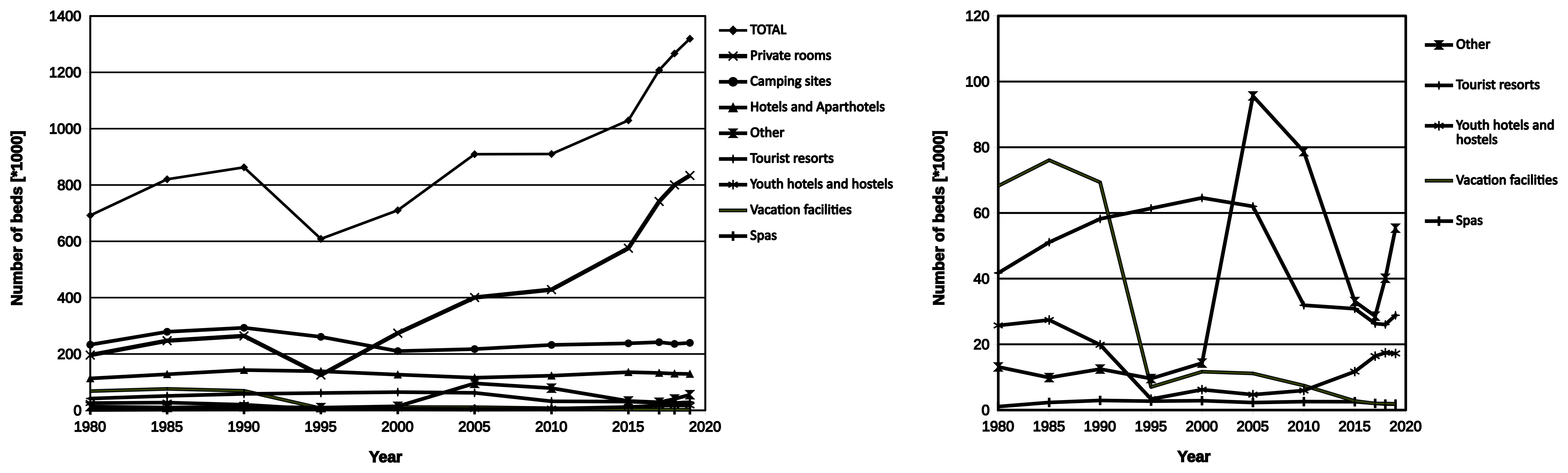
*all values are estimated or assumed and varied depending on test Layers data Identification of layers is the key point of the model. While sentiments are usually inert, in response to intense signals (e.g. disasters like epidemic or earthquake) they may change rapidly. For example recovery of frozen economy, thereafter lockdown will take some time due to aversion to the risk especially present in the tourist industry. Obviously, there is no rest in the presence of risk (excluding people adherent to risk). Identification of layers and their sensitivity to variety of signals is complex task, requiring not only access to raw data but trained experts and specialized software too. Luckily, this does not need to be done frequently as once computed layers do not change rapidly or change in the predictable manner.

Table 2. Attributes of layers used in econometric model.
Layer indexμ1μ2σ1σ2ρS, %
L1 (static)0,801,600,250,35–0,320
L2 (static)0,001,400,250,35–0,260
L3A (normal)0,200,600,250,300,520
L3B (epidemic)0,101,000,250,300,520
L3C (stimulated, 1)0,500,300,250,300,520
L3D (stimulated, 2)0,500,400,250,300,520

In order to study a numerical experiment three layers have been assumed in the try to model recovery from the lockdown. As layers are shaped according to bivariate correlated Gaussian distribution (1), they are fully defined by 6 parameters: standard deviations (σ1 and σ2), means (μ1 and μ2), correlation coefficient (ρ) i.e. components of covariance matrix, and share in the population (S). All values are presented in the Table 2. Probability density function f(x) of bivariate correlated Gaussian distribution is defined by the formula:

(1)
indecs-20-621-g3.gif
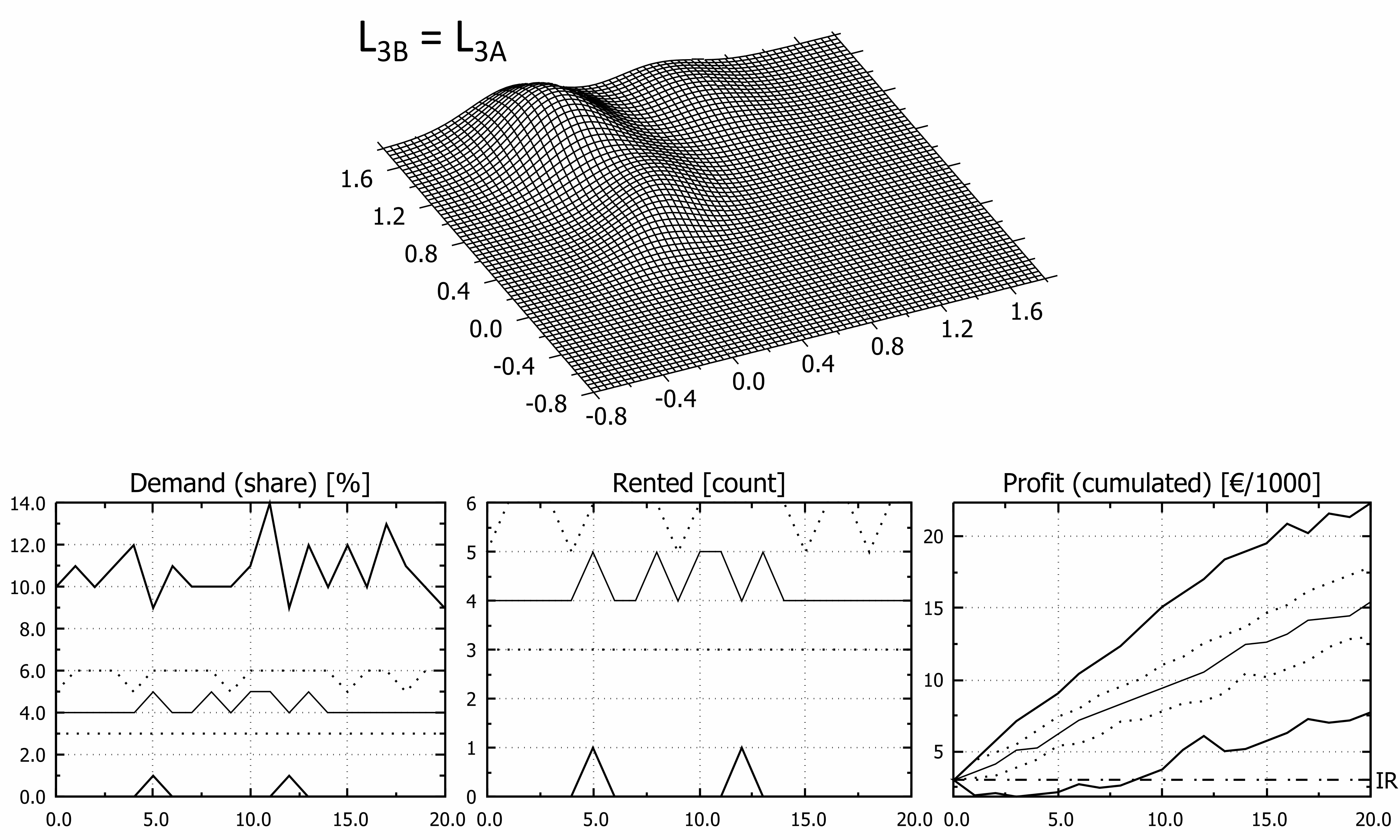
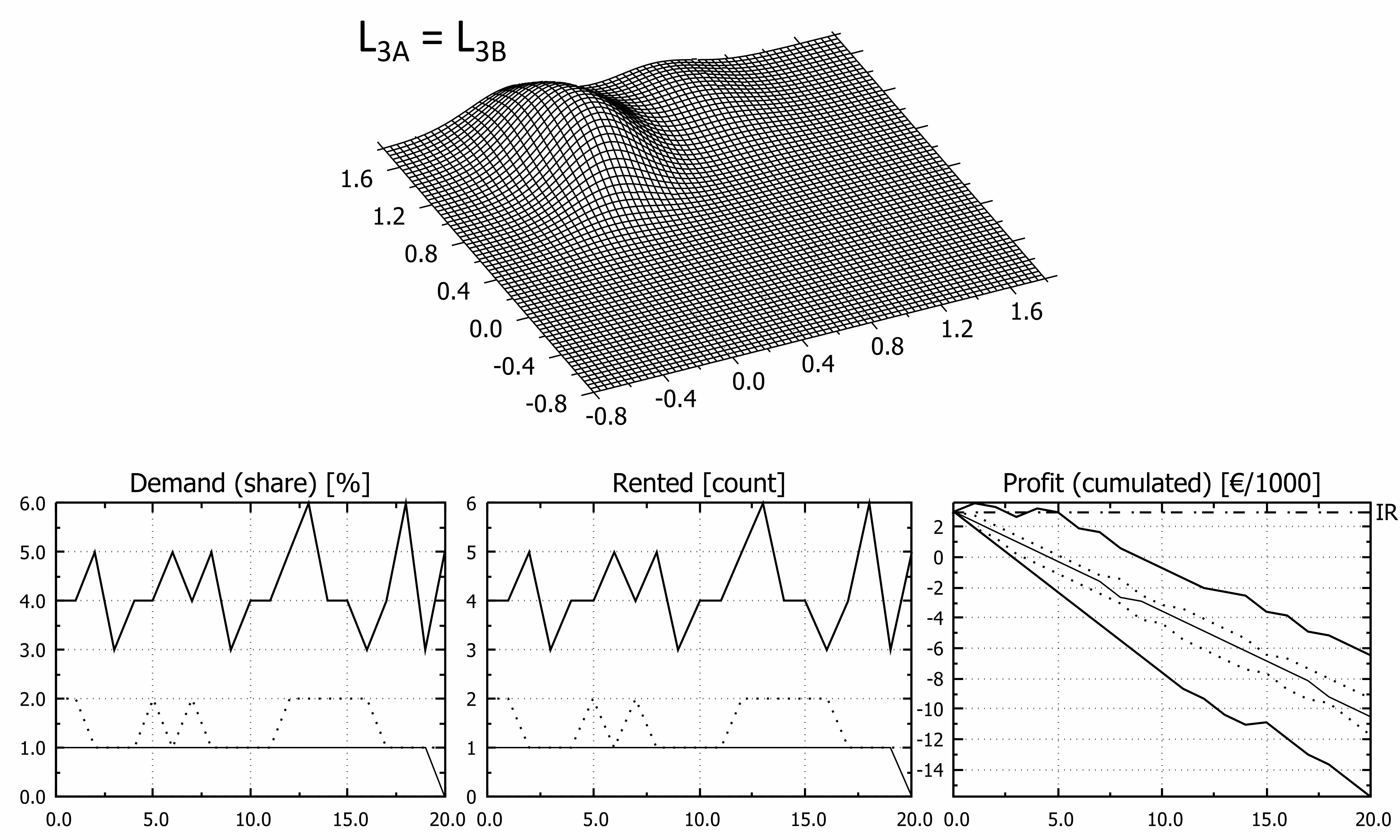
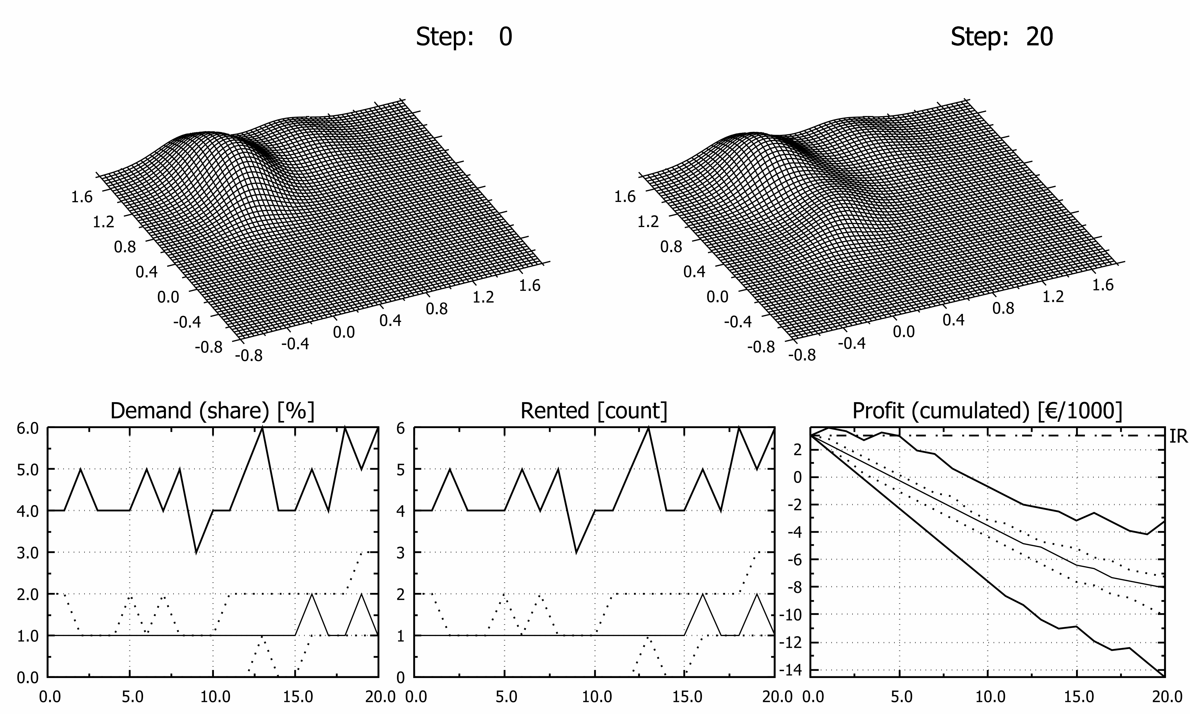
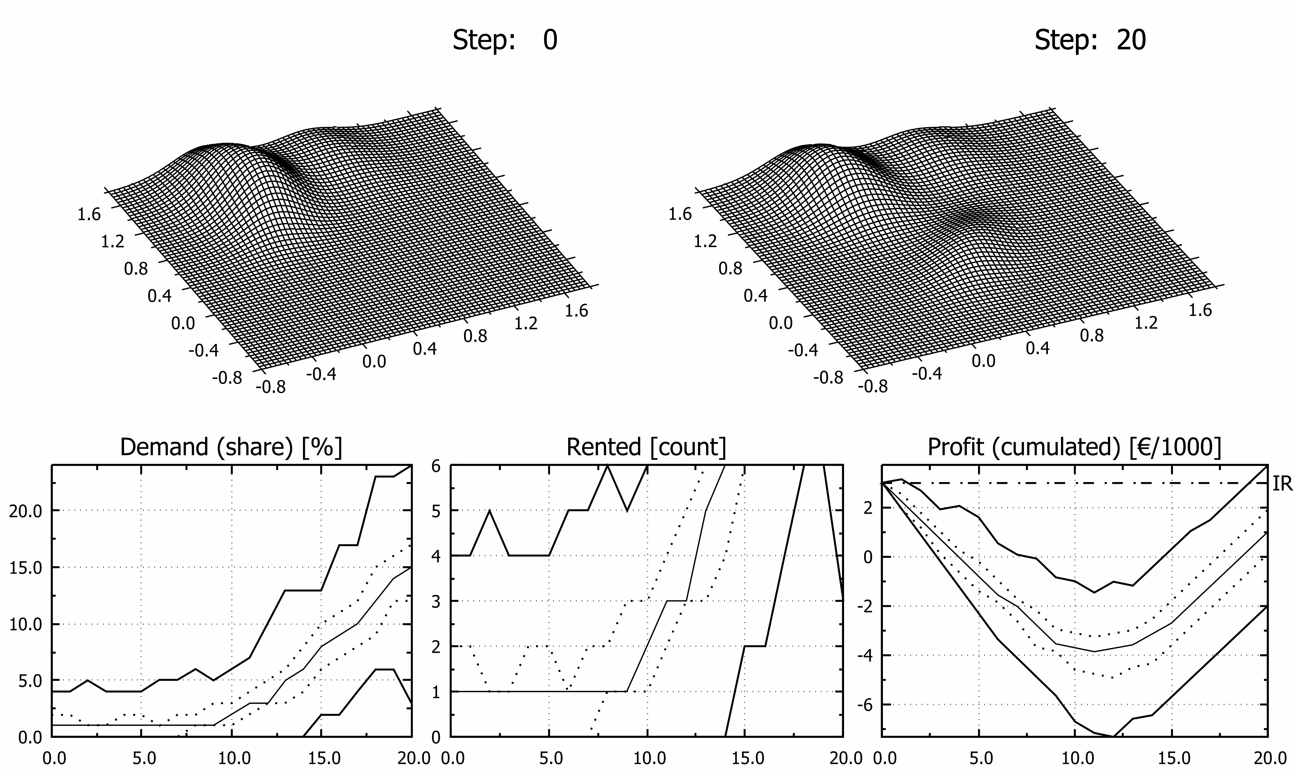
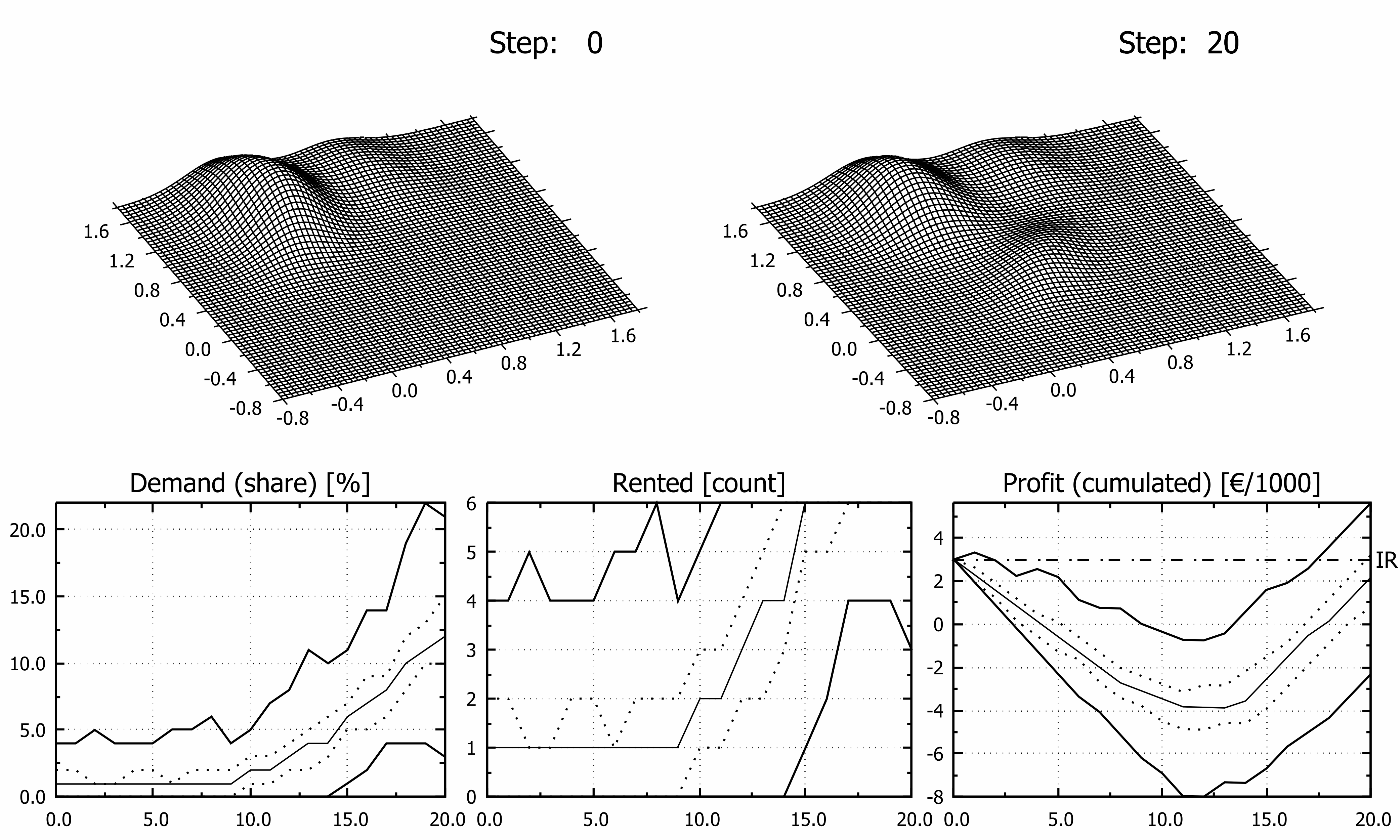
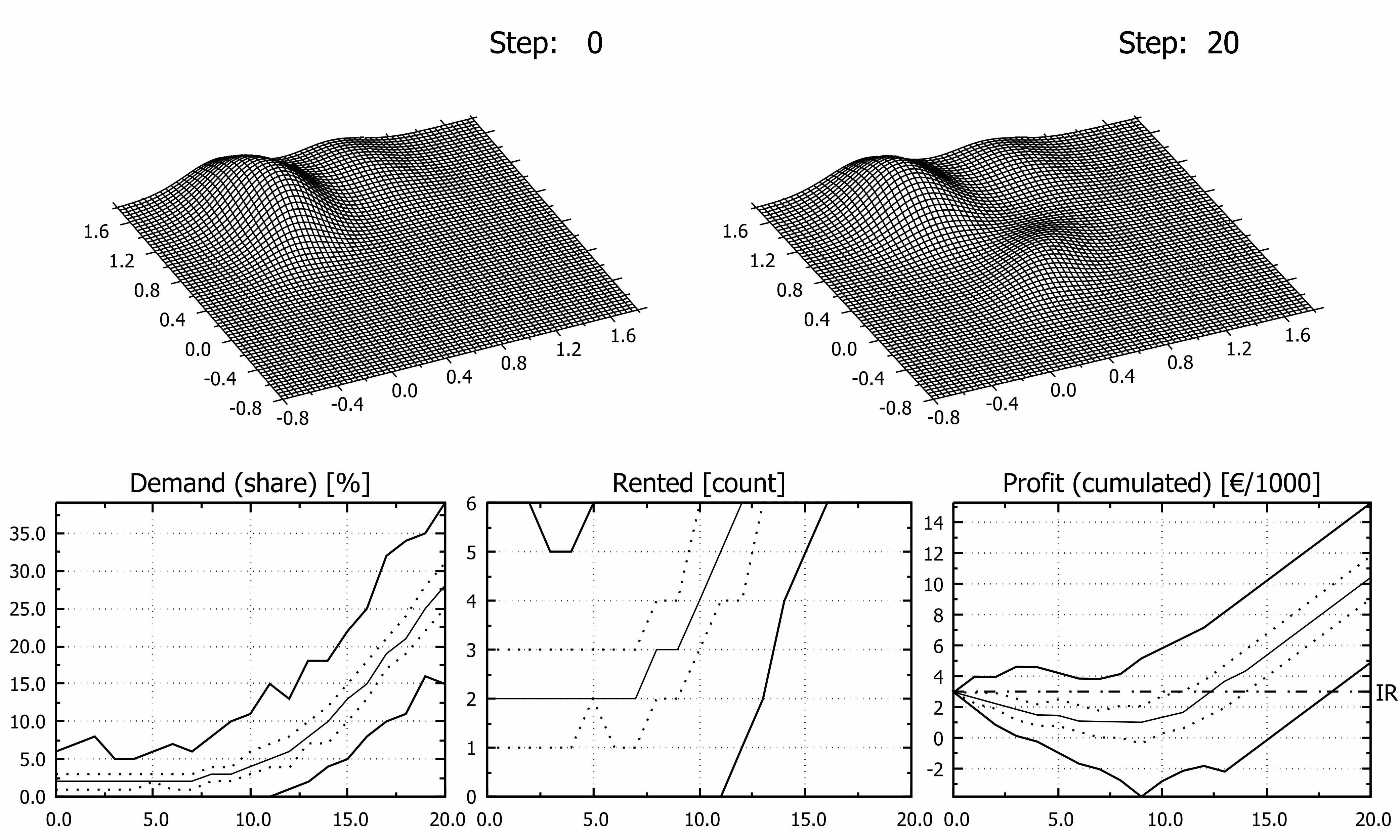
where x represents 2D point coordinates, µ denotes the mean (2D point as well) and C -1 is inverse of related covariance matrix. For higher dimensions formula stays the same excluding normalizing factor which depends on the dimensionality. In all scenarios Layer L3 migrates steadily from the selected initial state to the final state (ref. Table. 2). Uniform displacement per time step was hereby implemented nevertheless it may be step dependent. Layer L3A describes sentiments during normal season while layer L3B describes sentiments in the middle of first epidemic wave. The other layers have been assumed static in order to reduce number of variables in numerical experiments. However, in fully developed model they should “migrate” too and relative share of layers would probably change as well. Although variable, time dependent or stochastic displacement of the surface may be easily applied, it is out of scope and goal of this article as it introduces many new factors irrelevant to current discussion. It may be assumed that L1 and L2 layers represent domestic tourists not very favoring modelled destination, and less prone to foreign travel ban. Resulting Characteristic Surface may be symbolically denoted as CS = S1∙L1 + S2∙L2 + S3∙L3(t). Computer Program and Other Software Used Model has been implemented as C language console program (GCC compiler, tdm-1, v.5.1.0), source code is available for research groups on demand. According to the algorithm used, computing time scales linearly with the size of the population sample ‘N’ and number of repetitions ‘K’, thus BigO is of rank N×K. Use of regular laptop was sufficient for all calculations. Typical time of the single simulation was approximately 0,1 seconds over 20 week period (computed using clock() function), it was tested that 100 repetitions were optimal for convergence while not affecting significantly computing time. Charts have been prepared using gnuplot 5.4.135 and tuned using Inkscape 1.0236, if required. Obtained results are presented mainly on multi image (hybrid) charts. Images are arranged in two rows. Top row presents shape of Characteristic Surface before and thereafter migration of the monitored surface while a lower row shows estimated share of demand of monitored entity, number of apartments rented and cumulated profit respectively. In all charts lines presents minimum/maximum (solid bold line), lower and upper quartile (dotted line) and median (solid line) of depicted category. Vertical scales are expressed as percentage “Demand (share)” chart, as count of items in “Rented” chart and in thousands of euro (“Profit (cumulated)” chart). On the “Profit” chart black dashed horizontal line at y = 3, labelled ‘IR’ on secondary ‘Y’ axis depicts initial financial resources.
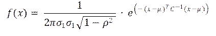
RESULTS

Figure 3. Simulation for the regular season, no migration of layers present.
indecs-20-621-g4.png
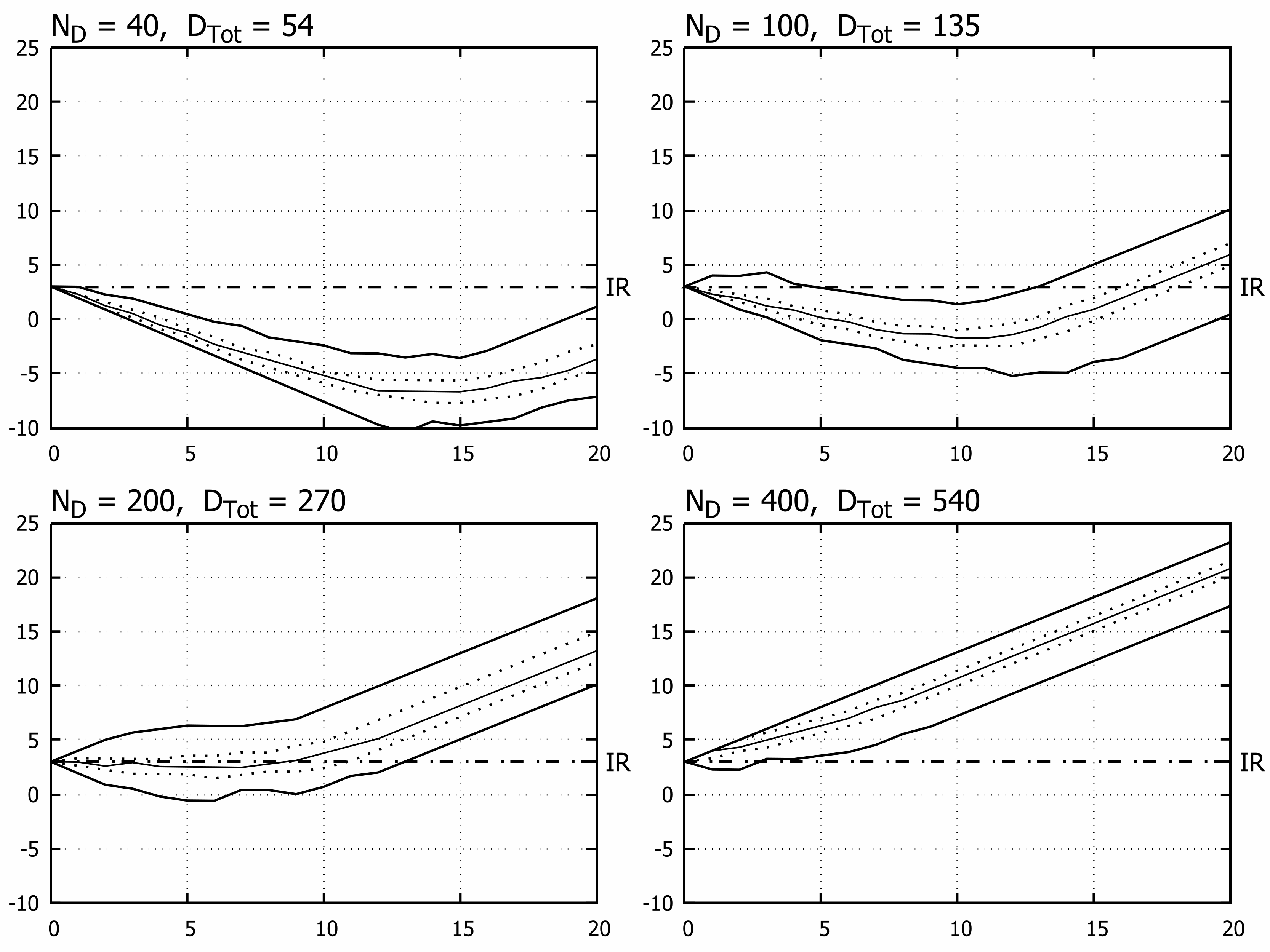
From a plenty of possible and tested scenarios seven were selected for the presentation of the model (Figures 3 to 9). Migration of the third layer from epidemic L3B state toward one of states L3A, L3C or L3D was assumed in all investigated cases but first two. Four more experiments were done in order to reveal influence of scale effect on estimated profit (Fig.10). Basic values of attributes of the model are presented in the Table 1. Maximum theoretical cumulated profit after whole season was 27 400€ (all apartments rented all the time) while the highest possible loss 21 200€ (no guests at all). In Figure 3 results of simulation assuming undisturbed season are presented, i.e. parameters of all disputed layers are constant over time. Specifically, this means that L3B layer was identical to L3A layer i.e. characteristic surface was the same in the course of simulation so it is drawn once in that Figure.
Figure 4. First wave of the epidemic, results of severe lockdown - all layers remains on “epidemic” L3B positions.
indecs-20-621-g5.png
Figure 5. Passive, nonstimulated recovery by spontaneous migration of the L3B layer to the pre-epidemic L3A state.Figure 5. Passive, nonstimulated recovery by spontaneous migration of the L3B layer to the pre-epidemic L3A state.
indecs-20-621-g6.png
As shown in Fig.3 median of demand’s share for analysed entity oscillates in the narrow band from 3 % to 6 % with 50 % probability (1st to 3rd quartile band), however maximum values incidentally reach 14 % and minimum values are down to 0 %. Hence, there is a noticeable uncertainty about profit. While median of cumulated profit is about 15 400 € on the end of the season, every value in the range from 13 000 € to 17 800 € approximately is possible with 50 % probability. In the worst possible scenario short term loss of initial resources in the beginning of the simulation is possible however barely probable. In the Figure 4. opposite case is discussed. Now the system, due to epidemic threat and restrictions, goes to epidemic layer L3B position and remains there, thus now L3A layer is identical with L3B layer. For this reason, as before, only one surface is shown in the picture. Additionally total demand in destination was reduced from pre-epidemic 200 units (e.g., individual tourists, families) to 90 only. Due to marginal demand from unaffected layers L1 and L2 demand for analysed entity is nonzero, however median equals 1 % most of the time and with probability 50 % demand’s share is less than or equal 2 %. Accordingly, no more than two apartments are rented, usually less. In effect owner suffers massive losses in the worst scenario at 15 800€ nearing maximum possible value. However median of loss is 10 500€ and 50 % of losses falls in the range 11 700-9 300 €. Results of the third experiment are presented in the Figure 5. Simulation starts just after the end of the first wave of epidemic and thus starting characteristic surface reflects negative sentiment (ref. Fig. 4), then third layer, L3B, (maybe the most adventurous tourists) starts moving toward its pre-epidemic location, L3A. Demand for the destination remains at epidemic level of 90 guests or families. Demand’s share remains at low level during whole simulation. Not only the minimum value remains at zero level but even maximum value is lower than capacity most of time. Accordingly, it is not possible to rent all apartments. Due to that cumulated profit drops until the end of simulation thus resources in the end would be smaller than in the beginning. Using layers metaphor, one may ask question what to do to speed‒up or intensify migration of third layer to its post-epidemic position in order to ensure faster recovery. There is no single and simple answer however. Popular solution is a discount supported by additional benefits (e.g., half board, fuel cost refoundation). This was studied in the next experiment. Effect of simulation is shown in the Figure 6. Intense shift of third layer (assumed attributes of L3C layer: μ1 = 0,50 and μ2 = 0,30) is attributed to aggressive price lowering by 25 % to 315 € (total demand for destination remained at 90) and benefits.
Figure 6. Overstimulated migration of the layer L3B to the state L3C after 25 % discount and benefits are offered.
indecs-20-621-g7.png
In simulation shown in Figure 6 demand’s share remains steady at low level but beginning from week 10th median starts rising and about week 14th exceeds capacity of the site. However minimum value remains at low level and minimum of demand is lower than capacity most of time. Despite that there is a small probability only that the host would not rent all apartments after week 15th. Accordingly, median of cumulated profit drops until 11th week then starts rising. Probability that final cumulated profit will be greater than initial resources (IR, Figure 6) is very small. This may mean that price lowering was too aggressive. Less aggressive option is popular discount “7 = 6” what means, that whole week is sold for price of six days. This time influence of price on final layer will be weaker, but incomes might be higher. Results of simulations are shown in the Figure 7, layer L3D (assumed attributes of L3D layer: μ1 = 0,50 and μ2 = 0,40, Table 2) was used as final layer. Less aggressive discount and lack of benefits make the offer less attractive, thus final μ2 is higher than in the previous example. Median of demand exceeds capacity around 15th week a week later than previously. Despite slower recovery of demand final profits are in 25 % of simulation greater than initial resources (IR line in Figure 7). However still there is a substantial risk of loss but currently with probability lesser than 25 %. This two results once again emphasize conclusion that all discounts should be based on precise risk assessment. Following two experiments test how restoring of initial demand would influence profits. Figure 8 shows effect of increasing of total demand by 50 %. Now probability of output greater than initial resources is remarkably greater than 75 % with no risk of final loss. Next, total demand reaches value of two hundred apartments from before the black swan. As shown in the Figure 9, now there is 100 % probability of not ending the season in red and 100 % probability of earning more money than initial resources. Moreover, positive results of recovery may be spotted started as early as from 8-9th week.
Figure 7. Moderate migration of the third layer from state L3B to the state L3D, “7 = 6” action engaged.
indecs-20-621-g8.png
Figure 8. Migration of the third layer from state L3A to the state L3D. “7 = 6” offer active and total demand increased by 50 %, up to 135 apartments.
indecs-20-621-g9.png
Figure 9. Migration of layer from state L3B to the state L3D. Total demand increased up to 200 apartments.
indecs-20-621-g10.png
The host may lower the price but as long as total demand for destination is lesser than total capacity this would not suffice. As shown allowing and encouraging tourists for coming in is crucial for recovery from the crisis. In the case of epidemic, one of possible methods is lowering price, but this reduces incomes too thus discount rates should be carefully estimated.
Figure 10. Scale effect influences results of simulation.
indecs-20-621-g11.png
Entities having the same attributes but in different locations may gain different profit depending on local offer and demand. Final, eighth experiment shows influence of scale effect on cumulated profit. Analyzed entity was virtually placed in three other destinations, having total offer (ND) and total demand (DTot) scaled. All values are estimated or assumed and varied depending on test, while total demand was assumed 50 % up from epidemic lowest level (DTot = 54, 135, 270, 540, respectively). As may be easily spotted not only stochastic fluctuations are smaller for larger system but profit is significantly higher as well. Facilities having the same attributes but located in different destinations may gain different profit depending just on local demand. In more populated destinations probability of profits is greater than in less. In similar circumstances an entity located in small destination may even suffer losses while profiting in larger. This is in accordance with common belief that it is easier to catch a fish in big river than in small stream.

DISCUSSION

Results presented in the previous section suggest that Characteristic Surface model is useful for modelling of economic output of a single small touristic entity in the era of pandemic. As the Model is founded on very weak assumptions, it is very general as well, and may be easily adopted to a variety of scenarios. Numerical efficiency of the Model is satisfactory and the Model itself scales linearly with number of repetitions and size of population involved. However, referential implementation of the Model may still be optimized by parallelization of computations for larger samples. According to results presented above, the Model exhibits ability to recreate typical business scenarios. The Model is sensitive to even small variations of the input data in all tested scenarios. Every parameter of the Model may be treated as a specific “degree of freedom” of its own variability range. Even after restricting number of options to M = 2, number of layers to L = 3 and omitting parameters of econometric model, number of possible combinations (Cartesian product) of remaining parameters: data of Layers (6×L, float numbers), population size N (positive integer), criterion function definitions (numerable, infinite), transfer function definitions (numerable, greater or equal 1) is infinite. For the selected case study on forecasting of recovery of Croatian tourism industry from epidemic, a few conclusions can be made. As increasing rate of rented apartments is crucial for cumulated profit, it may be assessed in a different manner. One possibility is that high social skills of the host, commonly addressed as emotional intelligence, may help increase attractiveness of a given entity over competitors. In terms of Characteristic Surface Model, this may be expressed as an additional push from social skills on layer L3 toward higher competitiveness (bigger µ1 values). Enhancement of the offer is possible as well. Markus et al.37 suggest that introduction of additional items like sports activities to the offer, may help increase sales. Applying discounts may increase the number of rented apartments but may deteriorate profit, thus it must be precisely computed. Surely, small revenues are always better than no revenues, however discounts must be calculated in order to maximize incomes. On the country level, there are more options available. In the first place, I would mention reducing stress and fear of potential guests, as there is no holidays in the presence of critical risk. This may be obtained by several means including (but not limited to) additional, low cost health assurance, increase of number of events for tourists – festivals, concerts or charming fisherman’s evenings, improving operation of highways toll system which currently is highly inefficient, safer organization of travelers resting places & fuel stations and strong support for domestic tourism. Of course, these remedies must be introduced by governmental agencies. Hypothesis may be formulated that post epidemic tourists are more adventurous then others and expect active offers, like nautical tourism, biking, climbing. This might be verified in dedicated research. As shown in the Results section, the Model allows for risk assessment for selected scenario. Furthermore, according to properties of MonteCarlo method, range of variability for computed outputs may be estimated.

CONCLUSIONS

Presented hereby method seems to be useful for the what-if analysis, giving quantitative answers thus allowing for decision making at known risk. While using of the model is rather simple, fine-tuning of crucial parts of the model might not be easy and may require a lot of additional research including variety of methods from simple A/B testing up to the most complex AI/ML. In particular, layers for the specific population may be subject of scientific research on its own. Results may be published by governmental agencies ready for use by individual entrepreneurs. Furthermore, besides new computational method, model introduces own descriptive language suitable for discussion concerning behaviour of analysed population. As assumptions the Model is built upon are very weak, it has almost no limitations. The main problems are proper identification and attribution of layers, determination of the response patterns (i.e. evolution of CS due to signals and time) and adoption of proper criterion function. Model easily scales with population size and may be applied to small, medium and large-scale systems. Although shown on the example of tourist industry, presented Model is universal and may be implemented for a variety of scenarios, including forecasting of general elections, demand on selected goods or number of visitors in National Park at a variety of weather conditions. Due to universal basics of the model another possible fields of implementation are sciences like physics or engineering. Possible areas of further development include methods of determination of Characteristic Surface, introduction of innovative transfer functions and development of time dependent criterion functions, including past experience simulation.

ACKNOWLEDGMENTS

The article was funded under subvention funds for the AGH University of Science and Technology in Krakow, Poland.

References

1 

Skalna L., et al.: Advances in Fuzzy Decision Making: Theory and Practice. Springer International Publishing, , 2015.http://dx.doi.org/10.1007/978-3-319-26494-3

2 

Čičak J., Vašiček D.: Determining the level of accounting conservatism through the fuzzy logic system. Business Systems Research,10(1),88-101, 2019.http://dx.doi.org/10.2478/bsrj-2019-0007

3 

Matsumoto M., Nishimura T.: ACM Transactions on Modelling and Computer Simulations. Special Issue on Random Number Generators1998.

4 

Matsumoto, M.:Mersenne Twister, computer program, Open Source,http://www.math.sci.hiroshima-u.ac.jp/~m-mat/MT/emt.html 4 9 2021.

5 

Opiła J., Skalna I.: Pseudorandom number generators in stochastic econometric models. In: Duda J.T. and Waszkielewicz W., eds.:Modern methods and techniques in management AGH Uczelniane Wydawnictwa Naukowo-Dydaktyczne, Cracow, pp.200-210 2006.

6 

Obućina, V.:Croatian tourism model – is it sustainable?, .https://www.obserwatorfinansowy.pl/in-english/croatian-tourism-model-is-it-sustainable 4 9 2021.

7 

Central Intelligence Agency:The world Factbook: Croatia, .https://www.cia.gov/the-world-factbook/countries/croatia 4 9 2021.

8 

Neufeld, D.:Visualizing the countries most reliant on tourism, .https://www.visualcapitalist.com/countries-reliant-tourism 4 9 2021.

9 

KNOEMA:Croatia - contribution of travel and tourism to GDP in constant prices of 2011.https://knoema.com/atlas/Croatia/topics/Tourism/Travel-and-Tourism-Total-Contribution-to-GDP/Real-contribution-of-travel-and-tourism-to-GDP 4 9 2021.

10 

Orsini, K. and Ostojić, V.:Croatia’s tourism industry: beyond the Sun and Sea.https://ec.europa.eu/info/publications/economy-finance/croatias-tourism-industry-beyond-sun-and-sea_en 4 9 2021.

11 

Moodys Analytics:Croatia - economic indicators.https://www.economy.com/croatia 4 9 2021.

12 

The World Bank:The World Bank in Croatia.https://www.worldbank.org/en/country/croatia/overview#3 4 9 2021.

13 

Croatia Week:Croatian PM announces package to help save jobs and economy.https://www.croatiaweek.com/croatian-pm-announces-package-to-help-save-jobs-and-economy 4 9 2021.

14 

Croatia Week:EC projects Croatia GDP to drop 9.6 % this year, return to pre-crisis level in 2022.https://www.croatiaweek.com/ec-projects-croatia-gdp-to-drop-9-6-this-year-return-to-pre-crisis-level-in-2022 4 9 2021.

15 

Croatia Week:Corona-free island of Rab records 80 % of last year’s tourist traffic.https://www.croatiaweek.com/corona-free-island-of-rab-records-80-of-last-years-tourist-traffic 4 9 2021.

16 

Croatia Week:Record 21 million tourists visit Croatia in 2019.https://www.croatiaweek.com/record-21-million-tourists-visit-croatia-in-2019 4 9 2021.

17 

Ministry of Tourism of Republic of Croatia:Tourism in figures 2018.https://www.htz.hr/sites/default/files/2019-09/HTZ%20TUB%20ENG_2018.pdf 4 9 2021.

18 

Ministry of Tourism of Republic of Croatia:Tourism in figures 2019.https://www.htz.hr/sites/default/files/2020-07/HTZ%20TUB%20ENG_2019.pdf 4 9 2021.

19 

Croatia Week:Croatia sees 99 % fewer tourists in April than last year.https://www.croatiaweek.com/croatia-sees-99-fewer-tourists-in-april-than-last-year 4 9 2021.

20 

Ministry of Tourism of Republic of Croatia:All in all, tourism did well in 2020, better results possible in 2021.https://mint.gov.hr/news-11455/htz-director-all-in-all-tourism-did-well-in-2020-better-results-possible-in-2021/22193 4 9 2021.

21 

Plecher, H.:Croatia: Youth unemployment rate from 1999 to 2020.https://www.statista.com/statistics/811946/youth-unemployment-rate-in-croatia 4 9 2021.

22 

Ministry of Tourism of Republic of Croatia:Nautical tourism responsible for this year’s tourism results, minister says.https://mint.gov.hr/news-11455/nautical-tourism-responsible-for-this-year-s-tourism-results-minister-says/21934 4 9 2021.

23 

Ministry of Tourism of Republic of Croatia:Only tourists from Poland, Kosovo and Turkey generated increase in nights in August.https://mint.gov.hr/news-11455/only-tourists-from-poland-kosovo-and-turkey-generated-increase-in-nights-in-august/21845 4 9 2021.

24 

Ministry of Tourism of Republic of Croatia:Croatia reports 54 % fall in tourist nights in Jan-Sept 2020.https://mint.gov.hr/news-11455/croatia-reports-54-fall-in-tourist-nights-in-jan-sept-2020/22062 4 9 2021.

26 

Opiła J.: An analysis of the evolution of consumer sentiment using the characteristic surface method. In Croatian.. In: Duda J.T,, ed.: Information systems and computational methods in management. In Polish. AGH Uczelniane Wydawnictwa Naukowo-Dydaktyczne, Kraków, pp.141-148 2005.

27 

Opiła J., Opiła C,, Cichowska J.: Emergency forecasting in microenterprise with the use of the extended surface method on the example of an agritourism farm. In Polish.. In: 9th International scientific conference Business management – theory and practice, WZ AGH, Kraków, pp.1-10 2008.

28 

Opiła J., Opiła C,, Cichowska J.: Forecasting of financial results of agrotourism farms by employing characteristic surface model Diagnosing the state of the environment, BTN, Bydgoszcz, pp.129-140 2008.

29 

Opiła J.: Visualization in a knowledge transfer process. In: ENTRENOVA-ENTerprise REsearch InNOVAtion Conference, Split,485-493 2018.

30 

Opiła J: Role of visualization in a knowledge transfer process. Business Systems Research,10(1),164-179, 2019.http://dx.doi.org/10.2478/bsrj-2019-0012

31 

Opiła J.: Employing of extended characteristic surface model for forecasting of demand in tourism. ENTRENOVA-ENTerprise REsearch InNOVAtion Conference,Split, pp.60-73, 2020.

32 

Kohavi R., Thomke S.H.: The surprising power of online experiments: getting the most out of A/B and other controlled tests. Harvard Business Review,95(5),74-82, 2017.

33 

Ramotowski, J.:Frank infects bank balance sheets not only in Central Europe. In Polish..https://www.obserwatorfinansowy.pl/tematyka/rynki-finansowe/bankowosc/frank-zaraza-bilanse-bankow-nie-tylko-w-srodkowej-europie 4 9 2021.

34 

Tepuš, M.M.:Housing finance models and standards in the republic of Croatia.http://housing-finance-networks.com/documents/doc.aspx?id=1631

35 

-:gnuplot.http://gnuplot.info 4 9 2021.

36 

-:inkscape.https://inkscape.org 4 9 2021.

37 

Markus Z.: Assessing tourist revisit intention through the sports and recreational services offered. Business Systems Research,10(2),141-150, 2019.http://dx.doi.org/10.2478/bsrj-2019-023


This display is generated from NISO JATS XML with jats-html.xsl. The XSLT engine is libxslt.