
Uvod
All environmental sciences rely heavily on methods that estimate the value of a dependent variable (Y) using a value for a related independent variable (X).
For instance, Freese (1964) noted that in the field of forestry, the volume of a tree (Y) may be described as a function of its breast height diameter (X), the strength of wood (Y) as a function of its specific gravity (X), and the cost of logging (Y) as a function of its proximity to hard-surfaced roads (X).
In agriculture, for example, soil organic matter (Y) may be expressed as a function of time (X), net photosynthesis (Y) can be related to irradiance (X), and respiration (Y) can be described as a function of temperature (X) (Archontoulis and Miguez, 2015).
Environmentalists might greatly benefit from a modeling tool that allows them to compare and assess a set of common regression models using the most frequently used fitting comparison criteria and conduct tests on all regression assumptions to see which one best fits their data.
Given Excel's popularity and ease of use, it would be an excellent option to provide a template for assessing a collection of such regression models.
Materijali i metode
Within the LineFit.xls template, we suggest conducting tests on 11 different regression models (SPSS, 2007), as shown in Table 1
Table 1. Models assessed with the LineFit template
Tablica 1. Modeli ocijenjeni pomoću predloška LineFit
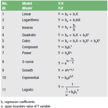
Linear regression is a useful statistical approach for estimating the value of a dependent variable (Y) through an independent variable (X). However, the following five assumptions must be satisfied before we are able to assess regression models' fit to our data:
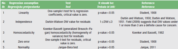
1. Linearity: bi regression coefficients should be statistically significantly different from zero.
2. Independence: Residuals should be independent, non-correlated.
3. Homoscedasticity: Residuals should have constant (homogeneous) variance across all Xi values.
4. Zero error: Residuals should have zero average.
5. Normality: Residuals should approximate a normal distribution.
Table 2 summarizes the five aforementioned assumptions along with the relevant literature.
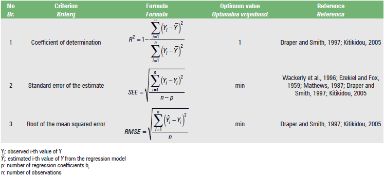
Table 3 provides three statistical comparison criteria and corresponding literature, for selecting the best fitted regression model for a given set of data
Table 2. Regression assumptions examined with the LineFit template
Tablica 2. Pretpostavke regresije ispitane u skladu s predloškom LineFit
Rezultati
LineFit.xls includes 13 spreadsheets. In the “data” spreadsheet, one can enter their own Y-X data in columns A and B, respectively (highlighted in blue). The amount of data can be up to 65535 entries (pairs of Y-X data). Summary statistics (count, mean, standard deviation, min, and max values) are given in cells D1:I4.
For demonstration purposes, columns A and B in the “data” spreadsheet are filled with a random number generator. By pressing the F9 key, one can observe all changes throughout the template.
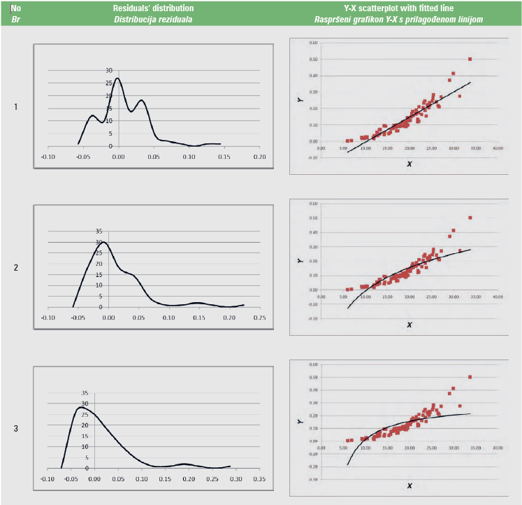
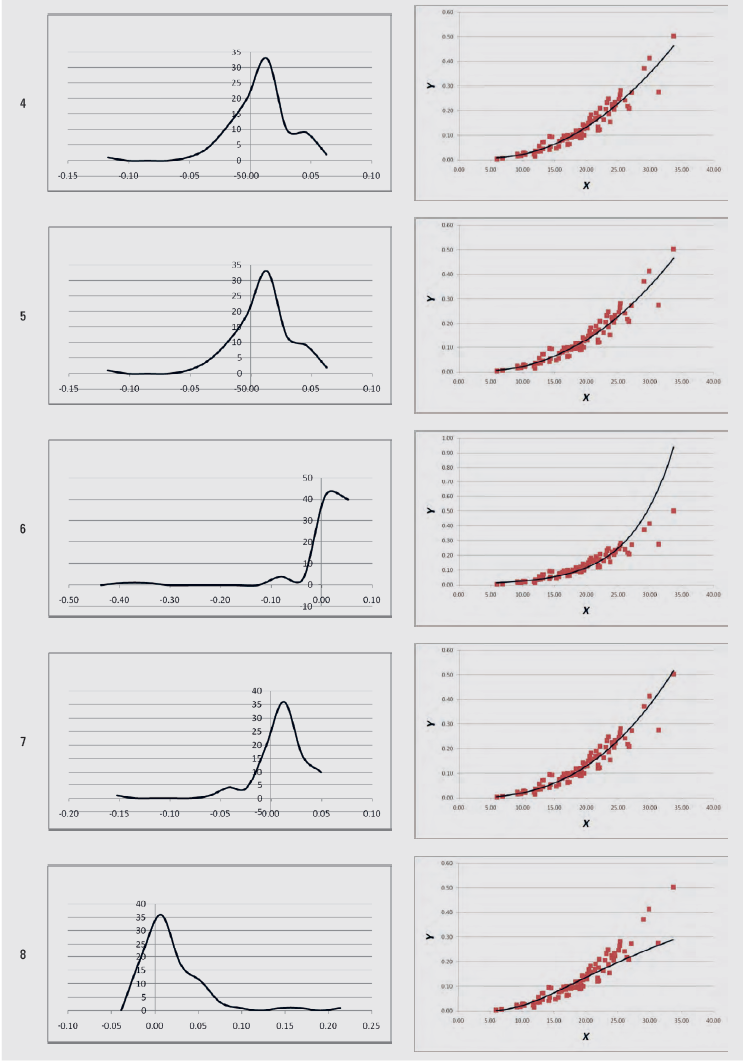
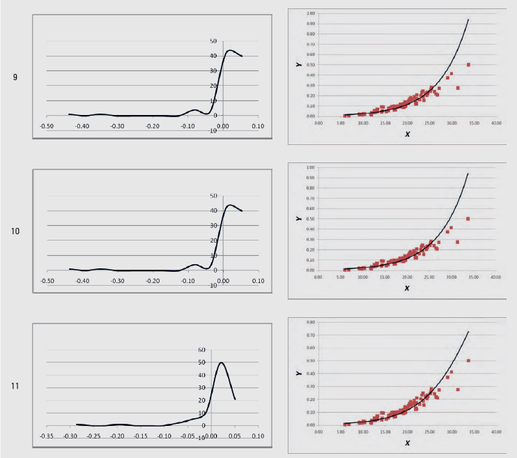
In the spreadsheets from “1” up to “11”, the statistics of Tables 2 and 3 are calculated, for each of the 11 regression models of Table 1. The linearity test is calculated across cells C5:F5, the independence test in cell M2, the homoscedasticity test in cell AO2, the zero error test in cell AM5, and the normality test in cell AM8. When the regression assumption is not satisfied, the font in these cells turns red. In addition, the graph of the residuals’ distribution and the Y-X scatterplot, along with the fitted line, are given for each of the 11 regression models.
An example of these graphs produced from volume (V, m3) – diameter at breast height (DBH, cm) data (Y-X data) (Softa, 2023) is given in Table 4.
Table 4. Graphs produced with the LineFit template from sample Y-X data
Tablica 4. Grafikoni proizvedeni pomoću predloška LineFit iz uzorka podataka Y-X
Regarding the statistical criteria for the comparison of the 11 regression models, the coefficient of determination R2 is calculated in cell J2, the Standard Error of the Estimate (SEE) in cell K2, and the Root of the Mean Squared Error (RMSE) in cell L2 in the corresponding spreadsheet for each of the 11 regression models.
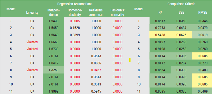
The regression assumptions listed in Table 2 and the statistical comparison criteria listed in Table 3 are both visible in their aggregated forms, in the “comparison” spreadsheet. At this point, the researcher has the opportunity to choose a particular regression model that will serve their needs in the most efficient way. When a regression assumption is not met, the font in these cells becomes red as well. Especially for the linearity test, when at least one regression coefficient is not statistically significantly different from zero, the “violated” message is displayed in red font. In the event that all regression coefficients are statistically significantly different from zero, the message “OK” is displayed.
Regarding the independence test, cells C3:C13 are conditionally highlighted. When a value is between 1.5 and 2.5, the cell is highlighted in dark green (optimum value), for a value between 1 and 1.5 or 2.5 and 3, the corresponding cell is highlighted in light green (acceptable value), and for a value >3 or <1, the corresponding cell is highlighted in yellow (the assumption of independence is not met).
The cells where the three statistical comparison criteria are calculated (i.e., the cells H3:J13) are highlighted on a graduated scale, from dark green (best values) to yellow (worst values).
For the data by Softa (2023), the results of the “comparison” spreadsheet are given in Table 5. Based on these results, one might decide (subjectively, not necessarily) that the best fitted model is the power (no 7) model:
V = 0.000046 · DBH2.6513
because the linearity, independence and residuals’ zero mean assumptions are not violated, and the comparison criteria have satisfactory values, compared with those of the other 10 models.
Table 5. Results of the “comparison” spreadsheet
Tablica 5. Rezultati proračunske tablice usporedbe (“comparison”)
Rasprava i zaključak
LineFit.xls is an all-in-one template whose outputs represent the behavior of eleven regression models, allowing any researcher to assess the fit of these models to their Y-X data. It is important to remember, however, that regression, as a parametric statistical process, may still perform pretty well even if some of the assumptions behind it are violated (Kitikidou et al., 2012; Kitikidou et al., 2013). Before rejecting a regression model because the assumptions are not met and choosing a non-parametric analysis, one should critically consider that non-parametric analyses employ rankings of values rather than the values themselves and hence cannot provide usable, quantitative estimations (Altman, 2009).
The LineFit.xls MS Excel template is available as a downloadable file on this journal's website to offer the scientific community an option to test and evaluate the most popular Y-X regression models with an all-in-one modeling tool.