1 Introduction
In books and textbooks on map projections, cylindrical, conic, and azimuthal projections are usually considered separately. It is sometimes mentioned that cylindrical and azimuthal projections can be interpreted as limiting cases of conic ones (Lee 1944,Kavrayskiy 1958, 1959, Jovanović 1983,Vakhrameyeva et al. 1986,Snyder 1987,Kuntz 1990,Canters 2022,Monmonier 2004,Serapinas 2005), but there are only a few attempts to prove it (Hinks 1912,Hoschek 1969,Daners 2012).
Kimerling (2010) in his blog introduced a way of thinking about similarities among projections − that seemingly distinct projections may actually be parts of a continuum of projections created by varying the parameters of a single pair of projection equations transforming the latitude and longitude coordinates on the sphere or ellipsoid into Cartesian coordinates on a flat projection surface. Such projection continuums are illustrated by animations that show the changes in the graticule and coastline as a certain projection parameter is varied systematically through a large range of values. Kimerling also provides animations showing the transition from conic to cylindrical or azimuthal projections.
In this paper, we will supplement the explanations and derivations ofHinks 1912, who applies Lambert's method of derivation (1772), although he does not mention Lambert.
The Lambert conformal conic projection is one of the most famous map projections. It is still used today in many countries. This projection was proposed by Lambert in his Notes and Supplements to the Establishment of Earth and Sky Maps published 250 years ago. The fourth subsection is A more general method of representing a spherical surface so that all angles preserve their sizes. That subsection is further divided and begins with §47 in which Lambert writes that the stereographic representation of the spherical surface, as well as Mercator nautical charts, have the property that all angles retain the size they had on the surface of the globe. In §48 Lambert derives the formula for the conformal projection of the unit sphere. After that he derived the Mercator projection as a limiting case of his conformal conic projection.
Hinks 1912 uses the same method as Lambert for the construction of a cylindrical projection as a limiting case of a conic projection. From the conic equidistant along the meridian (simple conic) he derives the cylindrical equidistant projection (in French projection plate carrée, in German quadratische Plattkarte). From the conformal conic (conic orthomorphic) he derives the conformal cylindrical projection (cylindrical orthomorphic – Mercator). For a simple equal-area projection with one standard parallel he does not give a derivation.
In this paper, we also give a derivation for the equal-area cylindrical projection as a limiting case of the equal-area conic projection. In addition, we give a derivation for the central perspective cylindrical projection as a limiting case of the central conic perspective projection.
It should be emphasized that Hinks defines a standard parallel as a parallel of true length: "One parallel, and sometimes a second, is made of the true length; that is to say, if the map is to be on the scale of one-millionth, the length of the complete parallel on the map will be one-millionth of the corresponding terrestrial parallel. This is called a Standard parallel." This definition does not correspond to today's understanding of distortions, according to which one should distinguish between standard parallels, equidistantly mapped parallels and parallels that have preserved their length in mapping.
Furthermore, Hinks implies in his derivations that a conic projection is a projection on a cone and that a cylindrical projection is a projection on a cylinder. In this paper, the conical and cylindrical projections are not projections on a cone or a cylinder whose surfaces are cut and developed into a plane, but rather mappings of the sphere directly into the plane. Exceptions are projections that are defined as mappings on the surface of a cone, as is the case with perspective projections.
Finally, we prove that it is not always possible to obtain a corresponding cylindrical projection from a conic projection, as one might conclude at first glance. Although very simple, it is the most important contribution of this article.
The equations of normal aspect conic projections are usually given in the polar coordinate system in the plane of the projection:
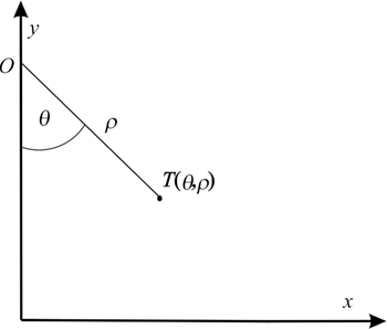
where φ ∈ (-π/2, π/2) and λ ∈ (-π, π) are the latitude and longitude, respectively, m the parameter, 0 < m≤1, θ and ρ the polar coordinates in the plane of projection (Fig. 1).
Figure 1. Point T and its polar coordinates θ and ρ. The origin O of the polar coordinate system is usually located on the y-axis of the rectangular coordinate system in the projection plane. / Slika 1. Točka Ti njezine polarne koordinate θ i ρ. Ishodište O polarnog koordinatnog sustava obično je smješteno na osi y pravokutnog koordinatnog sustava u ravnini projekcije.
A question arises: from a normal aspect conic projection given by the equations in the polar coordinate system in the projection plane (1), how can we, as a special limiting case derive the equations of the normal aspect cylindrical projection in the rectangular system in the projection plane
which will have analogous properties as the conic projection given by the equations (1). We are looking for a cylindrical projection (2), which is the counterpart of the conic one (1). For example, if the equal-area conic projection is given by the equations (1), how do the equations (2) of the equal-area cylindrical projection read? We will give the answer to that question in the next sections for equidistant, equal-area, conformal and perspective projections.
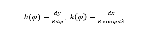
Before that, let us recall that the factors of the local linear scale along the meridian and the parallel, respectively, for conic projections of the sphere of radius R are (Snyder 1987)
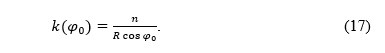
If k(φ0) = 1 holds for some φ0, then according to (3) we have
where we noted ρ0=ρ(φ0).
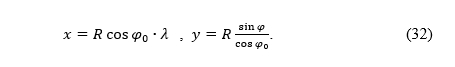
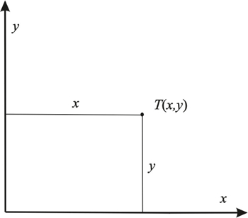
The equations of any normal aspect cylindrical projection are (2), where φ and λ are the latitude and longitude, respectively, n the parameter, usually 0 < n≤1, and x and y the rectangular coordinates in the plane of projection (Fig. 2).
Figure 2. Point T and its rectangular coordinates x and y. / Slika 2. Točka T i njezine pravokutne koordinate x i y.
If we write simply
we obtained the equations of the cylindrical projection from the equations of the conic projection (1) without any problems and without any recalculation. However, it can be easily shown that in this way some properties of the conic projection (1), e.g. equal-area or conformality, will not be preserved. Therefore, the procedure described by relations (5) does not provide the desired solution.
If we substitute m = 1 in (1), we will get the azimuthal projection equations:
If we substitute m = 0 in (1), we will get
which would mean that the entire sphere was mapped to a straight line or part of a straight line. So, to obtain a cylindrical projection from (1) with m = 0, we must add another condition to prevent the image of the sphere being compressed into a straight line. We can achieve this, for example, by requiring that one parallel that is equidistantly mapped by a conic projection also be equidistantly mapped by a cylindrical projection. In the following sections, we will show how a cylindrical projection can be obtained as a limiting case of a conic one using examples of equidistant along the meridian, equal-area, conformal and central perspective projections.
2 Projections equidistant along meridians
For the normal aspect conic projection of a sphere of radius R given by (1) to be equidistant along the meridians, the condition that the local linear scale factor along the meridians is equal to 1 must be met:
Integrating equation (8) gives
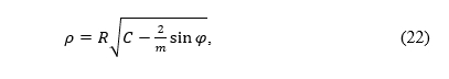
where C is a constant, C ≥ R*π/2 to make ρ ≥ 0 for each value of latitude. So, in the polar coordinate system, the equations of the conic projection that is equidistant along the meridians read:
Let us suppose that φ0 is the latitude of the equidistantly mapped parallel in that projection. Considering (4), we can write
and from there we have
and then
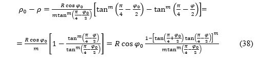
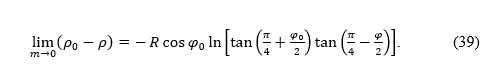
FollowingLambert (1772) andHinks (1912), let us consider the difference ρ0 -ρ. Although both ρ and ρ0 tend to infinity when m → 0, their difference is finite regardless of m:
This allows us to write the equations of a cylindrical projection equidistant along the meridians in a rectangular coordinate system in the projection plane
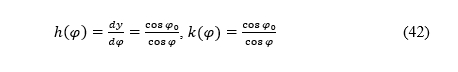
The factors of the local linear scale along the meridian and the parallel, respectively, for cylindrical projections of the sphere of radius R are (Snyder 1987)
Let us calculate
So, it is a cylindrical projection equidistant along the meridians. The local linear scale factor for that projection along the parallel to which the latitude corresponds φ0 is
For this parallel to be equidistantly mapped, k(φ0) = 1 should be true, i.e.
Thus, the equations of the normal aspect cylindrical projection equidistant along the meridians, which has the same standard parallel (φ0) as the conic projection (13) which is equidistant along the meridian, are
If we translate the image of the projection by the amount Rφ0 in the direction of the y axis, we will achieve that the image of the equator is on the coordinate axis x, as is usual in cartographic literature. So, the final equations of the normal aspect cylindrical projection equidistant along the meridian, which has the same equidistantly mapped parallel (φ0) as the conic projection (13) are
3 Equal-area projections
For the normal aspect conic projection of a sphere given by (1) to be equal-area, the condition that the product of the factors of the local linear scales along the meridian and along the parallel is equal to 1 must be satisfied, i.e. that
Integrating equation (21) gives
where C is a constant. Let us assume that C ≥ 2/m to make ρ real for each value of latitude. So, in the polar coordinate system, the equations of the equal-area conic projections read:
Let us suppose that φ0 is the latitude of the equidistantly mapped parallel in that projection. Considering (4), we can write
From (24) it follows
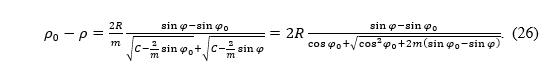
Now we can calculate
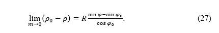
From (26) we obtain
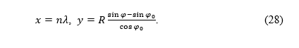
Now we can write the equations of equal-area cylindrical projection in a rectangular coordinate system in the projection plane
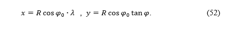
If we want the parallel corresponding to the latitude φ0 to be equidistantly mapped, then it should be n = Rcos(φ0), as we showed in the previous section (formula (18)). So, the final equations of the equal-area cylindrical projection are:
Let us check
Therefore,
If we translate the image of the projection by the amount Rtan(φ0) in the direction of the y axis, we will achieve that the image of the equator is on the coordinate axis x, as is usual in cartographic literature. So, the final equations of the normal aspect equal-area cylindrical projection, which has the same equidistantly mapped parallel (φ0) as the conic projection (23) are
4 Conformal projections
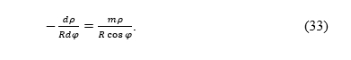
For the normal aspect conic projection given by (1) to be conformal, the condition is that the factors of the local linear scales along the meridians and along the parallels are equal, i.e. that the following holds
Integrating equation (33) gives
where C > 0 is a constant.
So, in the polar coordinate system, the equations of the conformal conic projections read:
Let us suppose that φ0 is the latitude of the equidistantly mapped parallel in that projection. Considering (4), we can write
From (36) it follows
Now we can calculate
When m → 0 then the last fraction is of the form 0/0. Applying l'Hospital's rule, we will get
Now we can write the equations of the conformal cylindrical projection in the rectangular coordinate system in the projection plane
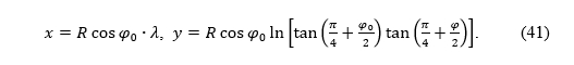
If we want the parallel corresponding to the latitude φ0 to be equidistantly mapped, then it should be n = Rcos(φ0) (formula (18)). The equations of the conformal cylindrical projection are:
Let us check for the projection (41):
Therefore,
If we translate the image of the projection by the amount
in the direction of the y axis, we will achieve that the image of the equator is on the coordinate axis x, as is usual in cartographic literature. So, the final equations of the normal aspect conformal cylindrical projection, which has the same equidistantly mapped parallel (φ0) as the conic projection (34) are
5 Perspective projections
The equations of the normal aspect central perspective projection on the cone can be written in the polar coordinate system in the form (Lapaine, Frančula 1992):
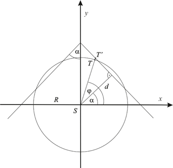
where α is a parameter that can be described geometrically as half the angle at the apex of the cone onto which the sphere is mapped and d the distance of the surface of the cone from the center (Fig. 3).
Figure 3. The gnomonic perspective conic projection. Point T' on the surface of the cone is the image of point T on the sphere of radius R. Points S, T and T' are collinear. See (Lapaine, Frančula 1992) / Slika 3. Gnomonska perspektivna konusna projekcija. Točka T' na plohi konusa je slika točke T na sferi polumjera R. Točke S, T i T' su kolinearne. Vidi (Lapaine, Frančula 1992)
Let us write
and calculate
If a → 0, then ρ and ρ0 tend to infinity, but their difference is finite
For the parallel corresponding to the latitude φ0 to be equidistantly mapped perspectively onto the cone according to formulas (45), considering (4) it should be true
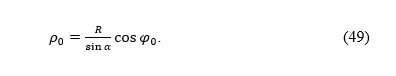
From (46) and (49) it follows
From (50) we can conclude that an equidistant mapped parallel in perspective conic projection exists if d ≤ R and that d = Rcos(φ0) holds for α = 0.
If we want the parallel corresponding to the latitude φ0 to be equidistantly mapped in the cylindrical projection, then it must be n = Rcos(φ0), as shown before.
Thus, the equations of the normal aspect central perspective on the cylinder in the rectangular coordinate system in the plane are
If we translate the image of the projection by the amountRsinφ0i in the direction of the y axis, we will achieve that the image of the equator is on the coordinate axis x, as is usual in cartographic literature. So, the final equations of the normal aspect perspective cylindrical projection, which has the same equidistantly mapped parallel (φ0) as the perspecitve conic projection (45) reads
6 Projections equidistant along parallels
For the normal aspect conic projection of the sphere of radius R given by (1) to be equidistant along the parallels, the condition that the local linear scale factor along the parallels is equal to 1 must be met:
From equation (51) the following is immediately obtained
Let us write
and calculate
When m → 0 then ρ0 - 0 →∞. In the theory of map projections, it is usually assumed that the functions defining map projections are real, single-valued, continuous, and differentiable functions of φ and λ in some domain and that their Jacobian determinant does not vanish (Tobler 1962). Therefore, in the described way, a cylindrical projection equidistant along the parallels cannot be obtained as a limiting case of a conic projection equidistant along parallels. Such a projection does not exist at all because in all normal aspect cylindrical projections all parallels are of equal length, and this is not the case on a sphere. This example proves that not all conic projections have a cylindrical limiting case as it seems at first glance.
7 Conclusion
Lambert (1772) derived the formula for the conformal conic projection. In the same publication, Lambert derived the equation of the Mercator projection as a limiting case of a conformal conic projection.Hinks (1912) used the same method as Lambert to construct a cylindrical projection as a limiting case of a conic projection. From the conic equidistant along the meridians (simple conic) he derives the cylindrical equidistant projection. For a simple equal-area projection with one standard parallel, Hinks does not give a derivation.
In this article, we give a derivation for the equal-area cylindrical projection as a limiting case of the equal-area conic projection. In addition, we give a derivation for the central perspective cylindrical projection as a limiting case of the central conic projection.
Furthermore, Hinks implies in his derivations that a conic projection is a mapping on a cone and that a cylindrical projection is a mapping on a cylinder. In this article, the conic and cylindrical projections are not projections on a cone or a cylinder whose surfaces are cut and developed into a plane, but mappings of the sphere directly into the plane. Exceptions are projections that are defined as mappings on the surface of a cone or plane, as is the case with perspective projections.
The main result of this paper is that it is not always possible to obtain a corresponding cylindrical projection as a limiting case from a conic projection, as one might conclude at first glance, and no one has noticed this so far. So, it is not advisable to interpret cylindrical projections as limiting cases of conic projections.
Acknowledgements
The author expresses his gratitude to anonymous reviewers for comments on an early version of this paper. The remarks allowed the author to make a much better paper.
1. Uvod
U knjigama i udžbenicima o kartografskim projekcijama obično se odvojeno razmatraju cilindrične, konusne i azimutne projekcije. Ponekad se spominje da se cilindrične i azimutne projekcije može tumačiti kao granični slučaj konusnih projekcija (Lee 1944,Kavrayskiy 1958, 1959, Jovanović 1983,Vakhrameyeva et al. 1986,Snyder 1987,Kuntz 1990,Canters 2022,Monmonier 2004,Serapinas 2005), a postoji samo nekoliko pokušaja da se to dokaže (Hinks 1912,Hoschek 1969,Daners 2012).
Kimerling (2010) (Hinks 1912,Hoschek 1969,Daners 2012).
Kimerling (2010) je u svojem blogu predstavio način razmišljanja o sličnostima među projekcijama − naizgled različite projekcije mogu zapravo biti dijelovi kontinuuma projekcija stvorenih variranjem parametara jednog para jednadžbi projekcija transformirajući koordinate geografske širine i dužine na sferi ili elipsoidu u kartezijeve koordinate u ravnini. Takvi su projekcijski kontinuumi ilustrirani animacijama koje pokazuju promjene u mreži i obalnoj crti, dok se određeni projekcijski parametar mijenja kroz veliki raspon vrijednosti. Kimerling također nudi animacije koje prikazuju prijelaz s konusne na cilindrične ili azimutne projekcije.
U ovom ćemo članku dopuniti objašnjenja i izvodeHinksa 1912 koji, iako Lamberta ne spominje, primjenjuje Lambertovu metodu (1772).
Lambertova je konformna konusna projekcija jedna od najpoznatijih kartografskih projekcija. I danas se koristi u mnogim zemljama. Tu je projekciju predložio Lambert u svojim Bilješkama i dodatcima za uspostavljanje karata Zemlje i neba objavljenima prije 250 godina. Četvrti je pododjeljak Općenitija metoda predstavljanja sferne površine tako da svi kutovi zadrže svoje veličine. Taj je pododjeljak dalje podijeljen i počinje s §47 u kojem Lambert piše da stereografski prikaz sferne površine, kao i Mercatorove pomorske karte, imaju svojstvo da svi kutovi zadržavaju veličinu koju su imali na površini globusa. U §48 Lambert izvodi formulu za konformnu projekciju jedinične sfere. Nakon toga je izveo Mercatorovu projekciju kao granični slučaj njegove konformne konusne projekcije.
Hinks 1912 se koristi istom metodom kao Lambert za konstrukciju cilindrične projekcije kao graničnog slučaja konusne projekcije. Iz konusne ekvidistantne projekcije uzduž meridijana (jednostavne konusne) on izvodi cilindričnu ekvidistantnu projekciju (na francuskom projection plate carrée, na njemačkom quadratische Plattkarte). Iz konformne konusne projekcije (conic orthomorphic) izvodi konformnu cilindričnu (cylindrical orthomorphic – Mercator). Za jednostavnu ekvivalentnu projekciju s jednom standardnom paralelom Hinks ne daje izvod.
U ovom članku dajemo i izvod za ekvivalentnu cilindričnu projekciju kao granični slučaj ekvivalentne konusne projekcije. Dodatno, dajemo izvod za centralnu perspektivnu cilindričnu projekciju kao granični slučaj centralne konusne perspektivne projekcije.
Treba naglasiti da Hinks standardnu paralelu definira kao paralelu stvarne duljine: "Jedna paralela, a ponekad i druga, ima pravu duljinu; to jest, ako karta treba biti u mjerilu jedan prema milijun, duljina cijele paralele na karti bit će milijunti dio odgovarajuće zemaljske paralele. To se zove standardna paralela." Ta definicija ne odgovara današnjem shvaćanju distorzija prema kojem treba razlikovati standardne paralele, ekvidistantno preslikane paralele i paralele koje su u preslikavanju sačuvale svoju duljinu.
Nadalje, Hinks u svojim izvodima implicira da je konusna projekcija projekcija na stožac, a da je cilindrična projekcija projekcija na valjak. U ovom radu konusne i cilindrične projekcije nisu projekcije na stožac ili valjak čije su plohe presječene i razvijene u ravninu, već preslikavanja sfere izravno u ravninu. Iznimke su projekcije koje su definirane kao preslikavanja na površinu stošca, kao što je slučaj s perspektivnim projekcijama.
Konačno, dokazujemo da nije uvijek moguće iz konusne projekcije dobiti odgovarajuću cilindričnu projekciju, kako bi se moglo zaključiti na prvi pogled. Iako vrlo jednostavan, to je najvažniji doprinos ovog članka.
Jednadžbe uspravnih konusnih projekcija obično su zadane u polarnom koordinatnom sustavu u ravnini projekcije:
gdje su φ ∈ (-π/2, π/2) i λ ∈ (-π, π) geografska širina, odnosno dužina, m parametar, 0 < m≤1, a θ i ρ polarne koordinate u ravnini projekcije (sl. 1).
Postavlja se pitanje: kako možemo iz uspravne konusne projekcije, zadane jednadžbama u polarnom sustavu u ravnini projekcije (1), izvesti jednadžbe uspravne cilindrične projekcije u pravokutnom koordinatnom sustavu u ravnini projekcije
Figure 1. Point T and its polar coordinates θ and ρ. The origin O of the polar coordinate system is usually located on the y-axis of the rectangular coordinate system in the projection plane

kao poseban granični slučaj, tako da ostanu sačuvana svojstva konusne projekcije zadane jednadžbama (1). Tražimo cilindričnu projekciju (2) koja je pandan konusne (1). Na primjer, ako je ekvivalentna konusna projekcija zadana jednadžbama (1), kako glase jednadžbe (2) ekvivalentne cilindrične projekcije? U sljedećem poglavlju dat ćemo odgovor na to pitanje za projekcije koje su ekvidistantne, ekvivalentne, konformne i perspektivne projekcije.
Prije toga prisjetimo se da su faktori lokalnih linearnih mjerila uzduž meridijana, odnosno paralela za konusne projekcije sfere polumjera R (Snyder 1987)
Ako vrijedi k(φ0) = 1 za nekiφ0, onda prema (3) vrijedi
gdje smo označili ρ0=ρ(φ0).
Jednadžbe bilo koje uspravne cilindrične projekcije su (2), gdje su φ i λ geografska širina, odnosno dužina, n parametar, obično 0 > n ≤ 1,, a x i y pravokutne koordinate u ravnini projekcije (sl. 2).
Ako jednostavno napišemo
dobit ćemo jednadžbe cilindrične projekcije iz jednadžbi konusne projekcije (1) bez ikakvih problema i preračunavanja. Međutim, lako se može pokazati da na taj način neka svojstva konusne projekcije (1), npr. ekvivalentnost ili konformnost, neće biti sačuvana. Dakle, postupak opisan relacijom (5) ne daje željeno rješenje.
Ako uvrstimo m = 1 u (1), dobit ćemo jednadžbe azimutne projekcije:
Ako uvrstimo m = 0 in (1), dobit ćemo
što bi značilo da je cijela sfera preslikana na pravac ili dio pravca. Dakle, da bismo iz (1) dobili cilindričnu projekciju uz m = 0, moramo dodati još jedan uvjet koji će spriječiti da se slika sfere stisne u pravac. To se može postići npr. zahtjevom da jedna paralela koja je ekvidistantno preslikana pri konusnoj projekciji bude također ekvidistantno preslikana pri cilindričnoj projekciji. U sljedećim ćemo poglavljima pokazati kako se može dobiti cilindrična projekcija kao granični slučaj konusne na primjerima ekvidistantne, ekvivalentne, konformne i perspektivne projekcije.
2. Projekcije ekvidistantne uzduž meridijana
Uspravna konusna projekcija sfere polumjera R zadana jednadžbama (1) ekvidistantna je uzduž meridijana ako je lokalno linearno mjerilo uzduž meridijana jednako 1, tj. ako vrijedi
Integriranje jednadžbe (8) daje
gdje je C je konstanta, C ≥ R*π/2 da bi bilo ρ ≥ 0 za sve vrijednosti geografske širine. Dakle, u polarnom koordinatnom sustavu jednadžbe konusne projekcije ekvidistantne uzduž meridijana glase:
Pretpostavimo da je φ0 geografska širina ekvidistantno preslikane paralele u toj projekciji. Uzevši u obzir (4), možemo napisati
i odatle imamo
i zatim
PremaLambertu (1772) iHinksu (1912), razmotrimo razlikuρ0 -ρ. Iako i ρ i ρ0 teže u beskonačnost kadm → 0, njihova je razlika konačna, neovisno o m:
To nam omogućava napisati jednadžbe cilindrične projekcije ekvidistantne uzduž meridijana u pravokutnom koordinatnom sustavu u ravnini projekcije
The factors of the local linear scale along the meridian and the parallel, respectively, for cylindrical projections of the sphere of radius R are (Snyder 1987)
Izračunajmo
Dakle, to je cilindrična projekcija ekvidistantna uzduž meridijana. Faktor lokalnog linearnog mjerila za tu projekciju uzduž paralele kojoj odgovara φ0 je
Da bi ta paralela bila ekvidistantno preslikana, trebalo bi biti k(φ0) = 1, tj.
Dakle, jednadžbe uspravne cilindrične projekcije ekvidistantne uzduž meridijana koja ima istu standardnu paralelu (φ0) kao konusna projekcija (13) su
Pomaknemo li sliku projekcije za iznos Rφ0 u smjeru osi y, postići ćemo da slika ekvatora bude na koordinatnoj osi x kao što je uobičajeno u kartografskoj literaturi. Dakle, konačne jednadžbe uspravne cilindrične projekcije ekvidistantne uzduž meridijana koja ima istu ekvidistantno preslikanu paralelu (φ0) kao konusna projekcija (13) su
3. Ekvivalentne projekcije
Uspravna konusna projekcija sfere zadana jednadžbama (1) ekvivalentna je ako je produkt faktora lokalnog mjerila uzduž meridijana i uzduž paralele jednak 1, tj. ako vrijedi
Integriranjem jednadžbe (21) daje
gdje je C konstanta. Pretpostavimo da je C ≥ 2/m kako bi ρ bio realan broj za svaku vrijednost geografske širine. Dakle, u polarnom koordinatnom sustavu jednadžbe ekvivalentne konusne projekcije glase:
Pretpostavimo da je φ0 geografska širina ekvidistantno preslikane paralele pri toj projekciji. Uzevši u obzir (4), možemo napisati
Iz (24) slijedi
Sad možemo izračunati
Iz (26) dobijemo
Sad možemo napisati jednadžbe ekvivalentne cilindrične projekcije u pravokutnom koordinatnom sustavu u ravnini projekcije
Ako želimo da paralela kojoj odgovara geografska širina φ0 bude ekvidistantno preslikana, tada mora biti n = Rcos(φ0) kao što je pokazano u prethodnom poglavlju (formula (18)). Dakle, konačne jednadžbe ekvidistantne cilindrične projekcije su:
Provjerimo
Dakle,
Pomaknemo li sliku projekcije za iznos Rtan(φ0) u smjeru osi y, postići ćemo da slika ekvatora bude na koordinatnoj osi x kao što je uobičajeno u kartografskoj literaturi. Dakle, konačne jednadžbe uspravne ekvivalentne cilindrične projekcije koja ima istu ekvidistantno preslikanu paralelu (φ0) kao konusna projekcija (23) su
4. Konformne projekcije
Da bi uspravna konusna projekcija zadana s (1) bila konformna, mora biti ispunjen uvjet da su faktori lokalnih mjerila uzduž meridijana i paralela međusobno jednaki, tj. da vrijedi:
Integriranje jednadžbe (33) daje
gdje je C > 0 konstanta.
Dakle, u polarnom koordinatnom sustavu jednadžbe konformne konusne projekcije su:
Pretpostavimo da je φ0 geografska širina ekvidistantno preslikane paralele u toj projekciji. Uzevši u obzir (4), možemo napisati
Iz (36) slijedi
Sad možemo izračunati
Kad m → 0, tada je posljednji razlomak oblika 0/0. Primjenom l'Hôpitalova pravila dobit ćemo
Sad možemo napisati jednadžbe konformne cilindrične projekcije u pravokutnom koordinatnom sustavu u ravnini projekcije
Ako želimo da paralela kojoj odgovara geografska širina φ0 bude ekvidistantno preslikana, tada mora biti Rcos(φ0) kao što je prije pokazano. Jednadžbe konformne cilindrične projekcije su:
Provjerimo za projekciju (41):
Dakle,
Pomaknemo li sliku projekcije za iznos
u smjeru osi y, postići ćemo da slika ekvatora bude na koordinatnoj osi x kao što je uobičajeno u kartografskoj literaturi. Dakle, konačne jednadžbe uspravne konformne cilindrične projekcije koja ima istu ekvidistantno preslikanu paralelu (φ0) kao konusna projekcija (34) su
5. Perspektivne projekcije
Jednadžbe uspravne perspektivne projekcije na konus mogu se napisati u polarnom koordinatnom sustavu u obliku (Lapaine i Frančula 1992):
gdje je α parametar koji se geometrijski može opisati kao polovina kuta u vrhu konusa na koji se sfera preslikava, a d udaljenost plašta stošca od središta (sl. 3).
Napišimo
i izračunajmo
Iako i ρ i ρ0 teže u beskonačnost kad a → 0, njihova je razlika konačna
Da bi paralela kojoj odgovara geografska širina φ0 bila ekvidistantno preslikana perspektivno na konus po formulama (45), treba prema (4) vrijediti
Iz (46) i (49) slijedi
Iz (50) možemo zaključiti da ekvidistantno preslikana paralela pri perspektivnoj konusnoj projekciji postoji ako je d ≤ R i da za α = 0 vrijedi d = Rcos(φ0).
Ako želimo da paralela kojoj odgovara geografska širina φ0 bude ekvidistantno preslikana pri cilindričnoj projekciji, tada mora bitin = Rcos(φ0), kao što je prije pokazano.
Dakle, jednadžbe uspravne centralne ili gnomonske cilindrične perspektivne projekcije u pravokutnom sustavu u ravnini projekcije glase
Pomaknemo li sliku projekcije za iznos Rsinφ0 u smjeru osi y, postići ćemo da slika ekvatora bude na koordinatnoj osi x kao što je uobičajeno u kartografskoj literaturi. Dakle, konačne jednadžbe uspravne konformne cilindrične projekcije koja ima istu ekvidistantno preslikanu paralelu (φ0) kao konusna projekcija (45) su
6. Projekcije ekvidistantne uzduž paralela
Da bi uspravna konusna projekcija sfere polumjera R zadana s (1) bila ekvidistantna uzduž paralela, faktor lokalnog linearnog mjerila uzduž paralela mora biti jednak 1:
Iz (53) neposredno slijedi
Napišimo
i izračunajmo
Kad m → 0, tada ρ0 - 0 →∞.. U teoriji kartografskih prijekcija obično se pretpostavlja da su funkcije koje definiraju kartografske projekcije realne, neprekidne i diferencijabilne funkcije od φ i λ na nekom području i da njihova Jacobijeva determinanta ne iščezava (Tobler 1962). Dakle, na opisani se način ne može dobiti cilindrična projekcija ekvidistantna uzduž paralela kao granični slučaj konusne projekcije ekvidistantne uzduž paralela. Takva projekcija ne može se dobiti ni na koji način, ona ne postoji jer su kod svih uspravnih cilindričnih projekcija slike paralela jednake duljine, a paralele na sferi nisu. Ovaj primjer pokazuje da nemaju sve konusne projekcije granični cilindrični pandan, kao što se na prvi pogled čini.
7. Zaključak
Lambert (1772) je izveo formulu za konformnu konusnu projekciju. U istoj publikaciji Lambert je izveo jednadžbu Mercatorove projekcije kao graničnog slučaja konformne konusne projekcije.Hinks (1912) se koristio istom metodom kao Lambert da bi konstruirao cilindričnu projekciju kao granični slučaj konusne. Iz konusne ekvidistantne uzduž mjeridijana (jednostavna konusna) izveo je cilindričnu ekvidistantnu projekciju. Za jednostavnu ekvivalentnu projekciju s jednom standardnom paralelom Hinks nije dao izvod.
U ovom članku izvodimo ekvivalentnu cilindričnu projekciju kako granični slučaj ekvivalentne konusne projekcije. Uz to izvodimo centralnu perspektivnu cilindričnu projekciju kao granični slučaj centralne konusne projekcije.
Nadalje, Hinks u svojim izvodima pretpostavlja da je konusna projekcija preslikavanje na konus i da je cilindrična projekcija preslikavanje na cilindar. U ovom članku konusne i cilindrične projekcije nisu projekcije na konus, odnosno cilindar, čije se plohe razrežu i razviju u ravninu, nego preslikavanja sfere izravno u ravninu. Izuzetak su projekcije koje su definirane kao preslikavanja na plohu konusa ili u ravninu, kao što je slučaj kod perspektivnih projekcija.
Glavni je rezultat ovog članka da nije uvijek moguće dobiti odgovarajuću cilindričnu projekciju kao granični slučaj konusne projekcije, kao što bi se moglo zaključiti na prvi pogled, a nitko to do sada nije uočio. Dakle, nije preporučljivo interpretirati cilindrične projekcije kao granične slučajeve konusnih projekcija.
Zahvala
Zahvaljujem anonimnim recenzentima na vrijednim komentarima. Njihove su mi primjedbe omogućile znatno poboljšanje prve inačice rukopisa.