
UVOD
Phenotypic differentiation of plants is directly influenced by various processes, such as the natural selection and the introduction of new alleles into a population through the gene flow (Antonovics 1968), as well as the appearance of newly formed characteristics through mutation (DeWoody et al. 2015) and the genetic drift (Eckert et al. 1996). The latter is notably pronounced when the effective population size is small, and the gene flow is limited (Tremblay and Ackerman 2001). Nevertheless, plant morphology is generally considered adaptive (Coleman et al. 1994; Westoby and Wright 2006) and plays an important role in populations’ persistence (Cavender-Bares 2019).
As sessile organisms, plants are constantly exposed to ever-changing environmental conditions that can cause differentiation in morphological and functional traits of plants (Bakhtiari et al. 2019). One of the most common strategies in combating environmental heterogeneity in plants is phenotypic differentiation via local adaptation, i.e., developing advantageous traits in local conditions (Kawecki and Ebert 2004; Gimeno et al. 2009). Another important aspect of phenotypic variation is phenotypic plasticity (Schlichting 1986), i.e., the ability of individual genotypes to produce different phenotypes when exposed to different environmental conditions. It is generally considered that plasticity and adaptive evolution are not mutually exclusive (Nicotra et al. 2010; Wright et al. 2016). Some traits or populations may respond through plasticity, others through evolution, and others through some combination of the two (Franks et al. 2014).
The presence of distinct morphotypes in woody species has been found to represent different adaptive and plastic responses to water stress (Ramírez-Valiente et al. 2010; Míguez-Soto et al. 2019; Bachofen et al. 2021), flooding (Silva et al. 2010), shading conditions (Abrams et al. 1992; Goulart et al. 2011), photoperiodism (Vaartaja 1961; Howe et al. 1995) and metabolism (Bertić et al. 2021). One of the most common outcomes of adaptation and plasticity is the great variation in leaf shape and size. Generally smaller leaves are advantageous in hot and dry habitats and at high intensities of solar radiation, while large leaves with less efficient energy exchange capacity are advantageous in cooler, moister and lower-irradiance habitats (Meier and Leuschner 2008; Tozer et al. 2015; Wang et al. 2019).
Species with vast distribution areas are usually characterized by being functionally and phenotypically diverse on the intraspecific level (Bakhtiari et al. 2019). One such species, covering diverse habitats and environmental conditions of Central and Southern Europe, is rosemary willow, Salix eleagnos Scop. These wide shrubs, or small trees, that reach up to 15 (20) m in height, are pioneers that stabilize the soil and have an outstanding ability to survive flooding and overburdening (Schütt and Lang 2014). Even though its distribution is scattered, the species covers a variety of habitats, ranging from alluvial, coarse-gravelled riverbeds near the mountains, to very dry, calcareous soils and sandy or stony steep slopes, at higher elevations (Hegi 1981; Dickmann and Kuzovkina 2014). Descriptions of the species are very scarce and include only few reports on the morphological characteristics (Krüssmann 1962; Hegi 1981). Leaves are usually described as lanceolate to narrow linear, up to 12 cm long, and 2 cm wide. Young leaves are pubescent on both sides, almost or completely glabrous on the upper side, dark green and slightly shiny. Petiole is up to 0.5 cm long, sparsely pubescent (Hegi 1981). The species is both wind- and insect-pollinated, dioecious, characterised by rapid growth rate, easy vegetative propagation and easy hybridization. Its small seeds are adapted to long-distance transport by air and water (Argus 1997; Dickmann and Kuzovkina 2014).
Due to broad ecological valence, rosemary willow is an excellent model species for providing insight into the influence of habitat and environment on morphological differentiation between morphotypes. Phenotypic responses to the environmental conditions have been previously reported for other willow species, such as S. alba L. (Özden Keles 2021), S. herbacea L. (Marcysiak 2012), S. viminalis L. (Drzewiecka et al. 2012; Gąsecka et al. 2012) and S. triandra (Tumpa et al. 2022). In this research, we examined leaf morphology of eight rosemary willow populations growing under diverse habitat and environmental conditions, in order to determine: (1) the extent to which leaf morphometric characteristics are influenced by environmental conditions; (2) the presence of various morphotypes of rosemary willow; (3) to get the first insight into the intra- and inter-population variability and population structuring of rosemary willow. The main hypothesis were: (1) leaf phenotypic variability is in a positive correlation with favourable environmental conditions; (2) diverse habitat conditions caused the emergence of different morphotypes of rosemary willow; (3) there is a significant intra- and inter-population variability based on leaf morphology.
MATERIJALI I METODE
Plant Material
Biljni materijal
Materials used in the analysis of morphological traits were collected during the summer of 2020. In total, eight populations were included in the study (Table 1; Figure 1A): three populations from the karstic sites (P1–Vela Draga; P2–Grobnik; P3–Crni Lug), and five populations from the riparian sites (P4–Kupica; P5–Bregana; P6–Ormož; P7–Legrad; P8–Krka). In each population, leaf samples for morphometric analysis were collected from 10 adult trees/shrubs, at least 20 m apart from each other, to minimize the probability of sampling of related individuals. A total of 10 short shoots with no signs of the presence of insects or diseases were collected from each individual shrub/tree. For the analysis, only the shoots within the outer, sunlit crown perimeter were considered. After the collection, the shoot samples were stored in the labelled plastic zip-lock bags. Zip-lock bags were then placed into a cooler bag to protect them from wilting and deforming. Afterwards, the plant material was taken to the herbarium, dried between newspapers and herbarized. Finally, a subsample of the shoots was taken for analysis, in form of randomly selected two leaves from the central part of the shoot, for a total of 20 leaves per tree/shrub. The plant material was stored and deposited in the herbarium at the Faculty of Forestry and Wood Technology of the University of Zagreb (DEND).
Table 1. Sampling sites, habitats, geographic coordinates, and multivariate diversity index (MDI) for eight studied Salix eleagnos populations.
Tablica 1. Istraživane populacije, tip staništa, geografske koordinate i multivarijatni indeks raznolikosti (MDI) za osam istraživanih populacija sivkaste vrbe.
* Values followed by the same letters are not significantly different at p > 0.05 according to Wilcoxon rank sum test.
* Vrijednosti nakon kojih slijede ista slova ne razlikuju se značajno pri p > 0,05 prema Wilcoxonovom testu sume rangova.
p —the significance level of differences in the average values of MDI between groups according to Kruskal-Wallis test.
p — razina značajnosti razlika u prosječnim MDI vrijednostima između skupina prema Kruskal-Wallis testu.
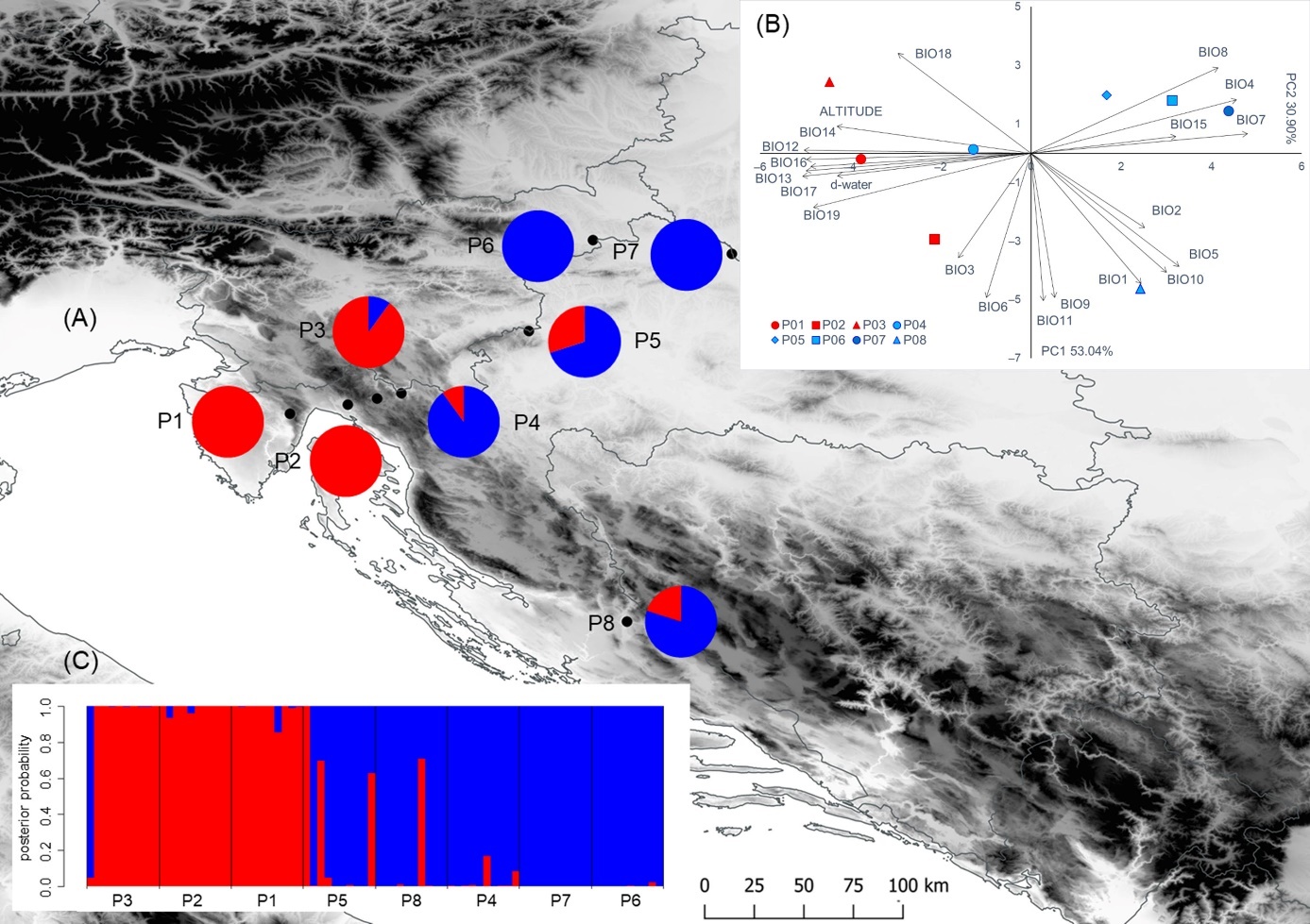
Figure 1. Results of the multivariate statistical methods and locations of the eight sampled Salix eleagnos populations. (A) Geographical distribution of the two groups of populations detected from K-means clustering method based on nine leaf phenotypic traits (the proportions of the membership of each population in each of the defined clusters are colour-coded: cluster A–red, cluster B–blue; (B) Biplot of the principal component analysis based on environmental variables; (C) Barplot with posterior probabilities of classification of each individual into each group from the results of the classification discriminant analysis. Populations: P1–Vela Draga; P2–Grobnik; P3–Crni Lug; P4–Kupica; P5–Bregana; P6–Ormož; P7–Legrad; P8–Krka.
Slika 1. Rezultati multivarijatnih statističkih metoda i lokacije osam istraživanih populacija sivkaste vrbe. (A) Geografska distribucija dviju skupina populacija dobivena metodom klasteriranja K-means na temelju devet morfoloških značajki listova (udjeli zastupljenosti svake populacije u svakom od definiranih klastera označeni su bojama: klaster A – crveno, klaster B – plavo; (B) Dijagram analize glavnih sastavnica na temelju značajki okoliša; (C) Barplot s posteriornim vjerojatnostima klasifikacije svake jedinke u svaku skupinu iz rezultata klasifikacijske diskriminantne analize. Populacije: P1–Vela Draga; P2–Grobnik; P3–Crni Lug; P4–Kupica; P5–Bregana; P6–Ormož; P7–Legrad; P8–Krka.
Studied morphological traits
Istraživane morfološke značajke
An MICROTEK ScanMaker 9800XL (MICROTEK, Hsinchu, Taiwan, TW) was used to scan the samples, along with a metric reference for subsequent measurement calibrations. The leaves were placed directly onto the scanner, adaxial side down, and scanned in greyscale at a resolution of 600 dpi. After scanning, the leaves were measured using WinFOLIA software (WinfoliaTM 2005), designed particularly for accurate measurements of leaf morphology. Data created by WinFOLIA analysis were stored in standard ASCII text files. A total of nine phenotypic traits were analysed, with six of them discerning leaf size: leaf area (LA); leaf length (LL); maximum leaf width (MLW); leaf length, measured from the leaf base to the point of maximum leaf width (PMLW); leaf blade width at 90% of leaf blade length (LWT); and petiole length (PL). The remaining three traits were used to describe the leaf shape: form coefficient (FC) and leaf angles LA1 and LA2. FC is a coefficient calculated as FC = 4piA/P2, where A=leaf area and P=leaf perimeter. The resulting value is a number between 0 (filiform object) and 1 (perfect circle). LA1 and LA2 are traits describing the base of the leaf blade by expressing the angles closed by the main leaf vein (the centre of the leaf blade) and the line connecting the leaf blade base to a set point on the leaf margin, at 10% (LA1) and 25% (LA2) of total leaf blade length.
Environmental data
Okolišne značajke
Data of the average climatic conditions for the period from 1970 to 2000, in the area of the studied populations, were obtained from the WorldClim 2 database with a spatial resolution close to a square kilometer (Fick and Hijmans 2017). The bioclimatic variables represent annual trends, seasonality and extreme or limiting environmental factors, useful when quantifying the effects of environmental conditions and climate changes on species distributions and phenotypic variability (O’Donnell and Ignizio 2012). All 19 bioclimatic variables were included in the analysis (Table 2): BIO1 (annual mean temperature); BIO2 (mean diurnal range (mean of monthly max temp–min temp)); BIO3 (isothermality (BIO2/BIO7) (×100)); BIO4 (temperature seasonality (standard deviation ×100)); BIO5 (max temperature of the warmest month); BIO6 (min temperature of the coldest month); BIO7 (temperature annual range (BIO5-BIO6)); BIO8 (mean temperature of the wettest quarter); BIO9 (mean temperature of the driest quarter); BIO10 (mean temperature of the warmest quarter); BIO11 (mean temperature of the coldest quarter); BIO12 (annual precipitation); BIO13 (precipitation of the wettest month); BIO14 (precipitation of the driest month); BIO15 (precipitation seasonality (coefficient of variation)); BIO16 (precipitation of the wettest quarter); BIO17 (precipitation of the driest quarter); BIO18 (precipitation of the warmest quarter); BIO19 (precipitation of the coldest quarter). In addition, two environmental variables were included in the study: distance-to-water and altitude. All variables were used to describe the environmental characteristics of the studied populations and to calculate the environmental distance matrix.
Table 2. Population habitats, distance to water, altitudes, and bioclimatic variables for the eight studied Salix eleagnos populations. Bioclimatic variables: BIO1 – BIO19 described in the text. Populations: P1-P8 as in Table 1.
Tablica 2. Udaljenost od vode (d-water), nadmorske visine i bioklimatske varijable istraživanih populacija. Bioklimatske varijable: BIO1 – BIO19 opisane u tekstu. Populacije: P1 – P8 kao u Tablici 1.
Leaf trait and population diversity
Varijabilnost svojstava listova i populacija
Descriptive statistics were calculated for each individual trait and for each population, with the goal of revealing the overall range of their variability (Sokal and Rohlf 2012). In addition, arithmetic means and coefficient of variations were calculated for the already defined groups, the karstic and riparian groups, and for the overall population sample. Hierarchical analysis of variance was used to determine the variability among the studied groups, between the populations, as well as between shrubs/trees within the populations. The populations’ factor was nested within the groups’ factor, whereas the shrub/tree’s factor was nested within the populations’ factor. In addition, differences of statistical significance, for all population pairs, were identified using the Fisher’s LSD multiple comparison test, at p≤0.05. Descriptive statistics and hierarchical analysis of variance were performed using the STATISTICA software package Version 13 (STATISTICA Version 13, 2018).
Population structure
Strukturiranost populacija
To identify the divergence and structure of the studied populations, multivariate statistical methods were used (McGarigal et al. 2000). Using K-means clustering method, based on nine leaf phenotypic traits, we revealed the number of clusters, which could present the differentiation between the studied populations most accurately (Douaihy et al. 2012). Populations were assigned to one cluster or were of mixed origin based on whether a specific population proportion was greater than or equal to 0.7 (one cluster) or less than 0.7 (mixed origin), respectively (Poljak et al. 2018).
Afterwards, the principal component analysis was conducted in order to reveal the interactions between the analysed variables, and to reduce all of the components to a lower number of factors. The biplot was constructed by two principal components showing analysed individuals and traits. In the conducted analysis, individuals were assigned to their populations, and groups “karstic” and “river” were marked by colour: karstic habitats in red and river in blue. In the same manner, groups were marked in all other multivariate analyses.
Discriminant analysis was performed to evaluate the utility and significance of the analysed leaf traits, revealing traits with greatest discriminatory power between the populations. The proportion of individuals correctly classified into the two studied groups of populations, the riparian and the karstic, was determined using classificatory discriminant analysis. Posterior probabilities of classification of each individual into studied groups from the results of the classification discriminant analysis were presented with a barplot.
The abovementioned multivariate statistical analyses were conducted using the “MorphoTools” R scripts in R v.3.2.2 (R Core Team, 2016) according to the manual by Koutecký (2015).
Morphological differentiation
Morfološka diferencijacija
Morphological differentiation was assessed by calculating the Euclidean distances between all pairs of individuals based on the scores of the first two principal components (PCs) considering nine leaf traits. The average Euclidean distances were calculated for each population and used as a multivariate diversity index (MDI) of a population. The Kruskal-Wallis test (among all populations) and the Wilcoxon rank sum test (between all possible population pairs) were performed using the STATISTICA software package Version 13 (STATISTICA Version 13, 2018), as was the Kruskal-Wallis test between karstic and riparian populations. In addition, an analysis of molecular variance (AMOVA; Excoffier et al. 1992) was performed using the Euclidean distance matrix (Karlović et al. 2009). Two-way AMOVA was used to partition total morphological variance between habitats (karstic vs. riparian), among populations within habitats, and within populations. Additional one-way AMOVAs were conducted to partition total morphological variance among and within populations of each habitat. Variance components were tested with 10,000 permutations in Arlequin ver. 3.5.2.2 (Excoffier and Lischer 2010).
Correlation between environmental, geographic, and morphometric data
Korelacije između okolišnih, geografskih i morfoloških značajki
Mantel test was used to evaluate the correlations between the multitrait differences between the populations. This test is regarded as the universal method for testing the relationship between multivariate data sets, expressed as dissimilarity matrices in biological problems, commonly used to quantify the degree of difference between individuals, populations, or species (Sokal and Rohlf 2012). In this study, three dissimilarity matrices were calculated in order to describe differences between the analysed populations: (1) morphometric differences as squared Mahalanobis distances between the pairs of populations; (2) environmental distances as the Euclidian distances between the population means for the first three PCs of the principal component analysis; and (3) geographic distance from the latitude and longitude of the sampling site. The significance level was assessed after 10,000 permutations as implemented in NTSYS-pc Ver. 2.21L (Rohlf 2009).
REZULTATI
Environmental differences among sampling sites
Okolišne razlike između područja uzorkovanja
In general, environmental variables included in this study were highly correlated (Table 3, Figure 1B). Principal component (PC) analysis, based on the correlation matrix, showed that the first four principal components had eigenvalues greater than 1 and together explained 96.52% of the variance (Table 3). The first principal component explained 53.04% of the total variance. A strong negative correlation with the first principal component (PC1) was found for eight environmental variables: BIO17 (precipitation of the driest quarter); BIO14 (precipitation of the driest month); BIO13 (precipitation of the wettest month); BIO12 (annual precipitation); BIO16 (precipitation of the wettest quarter); BIO19 (precipitation of the coldest quarter); altitude; and d-water. In addition, the same principal component was in a strong positive correlation with three bioclimatic variables: BIO7 (temperature annual range (BIO5-BIO6)); BIO4 (temperature seasonality (standard deviation ×100)); and BIO8 (mean temperature of the wettest quarter). The second principal component explained 30.90% of the total variance and was negatively correlated with six temperature-related variables: BIO11 (mean temperature of the coldest quarter); BIO6 (min temperature of the coldest month); BIO9 (mean temperature of the driest quarter); BIO1 (annual mean temperature); BIO10 (mean temperature of the warmest quarter); and BIO5 (max temperature of the warmest month). The first principal component separated the populations P1-P3 from higher elevations and karstic habitats characterized by higher precipitation, from other populations (P4-P8) from larger rivers, where lower precipitations were recorded. The second principal component revealed a notable bioclimatic sub-structure within the karstic and riparian populations. Of those, the northernmost sub-Mediterranean population P8 from the riparian group was characterized by high temperatures, whereas population P3 from the karstic group was characterized by the lowest temperatures.
Table 3. Pearson’s correlation coefficients between environmental variables and scores of the first four principal components. Bioclimatic variables BIO1-BIO19 as in Table 2.
Tablica 3. Pearsonovi koeficijenti korelacije između okolišnih značajki i vrijednosti prve četiri glavne sastavnice. Bioklimatske varijable BIO1 – BIO19 kao u Tablici 2.
Leaf traits analysed and population diversity
Istraživana svojstva listova i raznolikost populacija
Overall, correlations between measured traits were positively or negatively correlated with each other at a statistically significant level ( p˂0.01). In general, leaf size-related variables were positively correlated in almost all pairs examined (Table 4). A strong positive correlation ( r > 0.70) was found in nine out of 36 pairs examined. Furthermore, weak negative relationship between leaf size and shape was statistically significant in only several cases: FC demonstrated a negative correlation with three traits (LL, PMLW, PL); LA2 with three traits (LL, PMLW, PL); and LA1 with two (PMLW, PL). In addition, the results showed that there were no significant correlations between the four trait pairs.
Table 4. The results of correlation analysis between leaf traits. The results are presented as correlations on all 80 individuals. Morphometric traits analysed: LA—leaf area; FC—form coefficient; LL—leaf blade length; MLW—maximum leaf width; PMLW—leaf blade length measured from the leaf base to the point of maximum leaf width; LWT—leaf blade width at 90% of the leaf blade length; LA1—angle closed by the main leaf vein and the line defined by the leaf blade base and the point on the leaf margin, at 10%; LA2—angle closed by the main leaf vein and the line defined by the leaf blade base and the point on the leaf margin, at 25%; PL—petiole length.
Tablica 4. Rezultati korelacijske analize između istraživanih svojstava listova. Rezultati su prikazani kao korelacije između svih 80 jedinki. Istraživane morfološke značajke: LA – površina plojke; FC – koeficijent oblika; LL – duljina plojke; MLW – maksimalna širina plojke; PMLW – duljina plojke mjerena od baze lista do točke najveće širine plojke; LWT – širina plojke na 90 % duljine plojke; LA1 – kut zatvoren glavnom lisnom žilom i linijom definiranom bazom plojke i točkom na rubu plojke, na 10 %; LA2 – kut zatvoren glavnom žilom lista i linijom definiranom bazom plojke i točkom na rubu plojke, na 25 %; PL – duljina peteljke.
*** significant at p < 0.001, ** significant at 0.001 < p < 0.01, * significant at 0.01 < p < 0.05, ns depicts non-significant values ( p > 0.05)
Basic data, i.e., mean values and coefficient of variations of each trait, are given in Table 5 for populations, habitats and the overall populations’ sample. Coefficients of variations for the overall sample were high for all of the analysed traits, with all traits having CV above 20%. Extremely high variability, with CV above 30%, was noted for LA (CV=39.24%), PL (CV=37.19%), and LWT (CV=30.83%).
For most traits, mean values of karstic populations were smaller than those of riparian populations. In other words, karstic populations were characterized by smaller, more elongated leaves with more acute leaf blade base. Regarding individual populations , in the karstic group populations P1 and P2 stood out. Population P1 was characterized by the longest leaves and the most acute leaf blade base, whereas population P2 stood out by having the smallest leaves. In the riparian populations’ group, P7 stood out by having the roundest leaves, and largest leaves characterized populations P4 and P5.
Table 5. Results of the descriptive statistical analysis for the studied populations and morphometric traits. Morphometric traits’ acronyms as in Table 4. Descriptive parameters: M—arithmetic mean and CV—coefficient of variation (%). Populations: P1-P8 as in Table 1.
Tablica 5. Rezultati deskriptivne statističke analize za istraživane populacije i morfološka svojstva. Akronimi istraživanih morfoloških svojstava kao u Tablici 4. Deskriptivni pokazatelji: M – aritmetička sredina; CV – koeficijent varijabilnosti (%). Populacije P1 – P8 kao u Tablici 1.
The results of the analysis of variance are summarized in Table 6. Statistically significant differences between the analysed groups, karstic and riparian, were confirmed for five out of nine measured traits: LA, LL, MLW, LWT and LA1. Populations within the groups differed in seven out of nine traits, with no differences found for LA and LWT. Individuals within the populations were statistically different for all measured traits. As expected, intrapopulation variability was higher than the interpopulation variability, for most traits. However, for six out of nine traits, the highest percentage of the total variability was represented by residue component, i.e., leaf variability on the individual shrub/tree. The exception to this rule were three traits (LA, MLW, LWT), which demonstrated the highest percentage of the overall variability for differences among the two groups, i.e., the two morphotypes.
Table 6. Hierarchical analysis of variance. Morphometric traits’ acronyms as in Table 4.
Tablica 6. Rezultati hijerarhijske analize varijance. Akronimi istraživanih morfoloških svojstava kao u Tablici 4.
*** significant at p < 0.001, ** significant at 0.001 < p < 0.01, * significant at 0.01 < p < 0.05, ns depicts non-significant values ( p > 0.05)
*** značajno pri p < 0,001, ** značajno pri 0,001 < p < 0,01, * značajno pri 0,01 < p < 0,05, ns prikazuje neznačajne vrijednosti ( p > 0,05)
Since the variance analysis revealed significant differences between the populations for most of the researched traits, a post-hoc testing by Fisher’s multiple tests (LSD) was conducted for all population pairs, in order to determine the exact number of populations differing significantly for each individual trait (Table 7). Significant differences were found between almost all population pairs. The most pronounced differences were found between the karstic and the riparian populations, as well as between the population P7 and all other populations. Populations P4 and P5, and P6 and P8 did not demonstrate a single significant difference, and a single statistically significant difference was noted for the following population pairs: P2 and P3; P5 and P6; P5 and P8. The majority of population pairs demonstrated differences for six or more traits.
Table 7. Results of Fisher’s LSD test. Morphometric traits’ acronyms as in Table 4. Populations as in Table 1.
Tablica 7. Rezultati Fisherovog LSD testa. Akronimi morfoloških svojstava kao u Tablici 4. Populacije kao u Tablici 1.
Population structure
Strukturiranost populacija
As previously indicated, significant variations between different populations, according to their environmental origin, have been confirmed by the multivariate statistical analysis as well. As a result, the researched populations were divided optimally into two clusters, by K-means analysis (Figure1A), with clusters corresponding to the predefined population groups, in karstic and riparian habitats. From the total of 80 individuals, 35 were assigned to Cluster A, and the remaining 45 to Cluster B. Cluster A encompassed individuals from populations P1-P3, found on the karstic sites, and Cluster B encompassed the riparian populations of P4-P8. All of the P1 and P2 individuals were assigned to Cluster A, whereas all individuals from P6 and P7 were assigned to Cluster B. None of the populations demonstrated mixed origin, i.e., all tested populations demonstrated proportion of membership above 0.7. A similar environmental gradient was also visible from the PCA and CDA results.
In PCA, the first principal component axis indicated differentiation of samples from karstic and riparian sites (Figure 2). Only one individual from the karstic populations grouped with the riparian population group, whereas only five individuals from riparian populations grouped with the karstic population group. The first two components had the eigenvalues above 1 and explained 87.98% of the total variability (Table 8). The first principal component was highly positively correlated to three traits, whereas the second principal component correlated highly positively with two, and highly negatively with two traits.
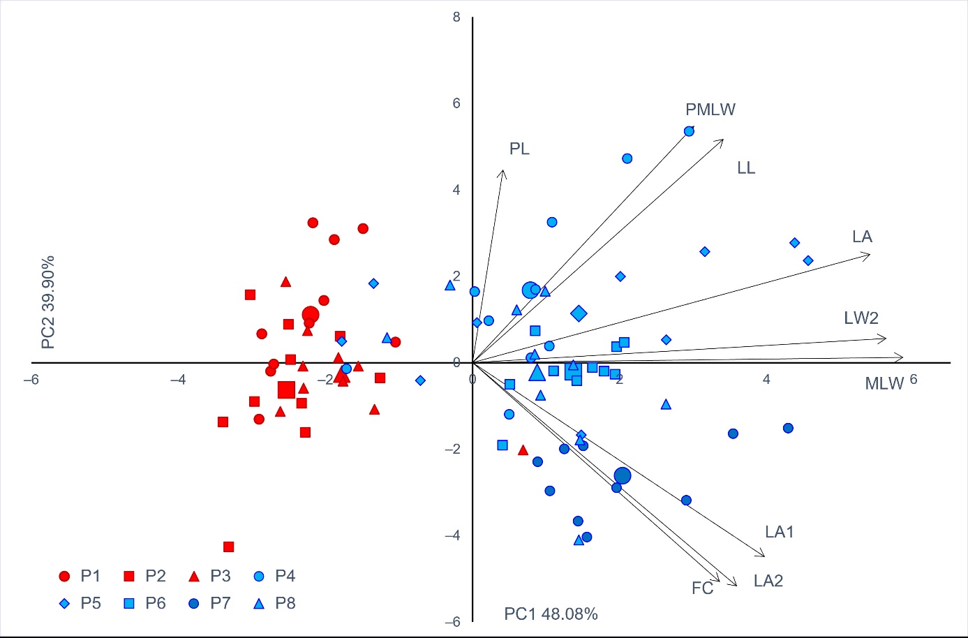
Figure 2. Biplot of the principal component (PC) analysis based on nine leaf phenotypic traits in the studied Salix eleagnos populations. Each individual tree is indicated by a small sign, while the population barycenters are represented by larger ones. The colour of the signs is related to the two groups of populations detected from K-means clustering method (cluster A–red, cluster B–blue). Morphometric traits’ acronyms as in Table 4. Populations as in Table 1.
Slika 2. Dijagram analize glavnih sastavnica (PC) na temelju devet morfoloških značajki listova u istraživanim populacijama sivkaste vrbe. Svaki pojedini grm označen je malom oznakom, dok su populacijski baricentri predstavljeni većim oznakama. Boja oznaka povezana je s dvije skupine populacija dobivenih metodom klasteriranja K-means (grupa A – crvena, skupina B – plava). Akronimi morfoloških svojstava kao u Tablici 4. Populacije kao u Tablici 1.
Table 8. Pearson’s correlation coefficients between morphometric traits and scores of the first three principal components. Morphometric traits’ acronyms as in Table 4.
Tablica 8. Pearsonovi koeficijenti korelacije između morfoloških svojstava i prve tri glavne sastavnice. Akronimi istraživanih morfoloških svojstava kao u Tablici 4.
In CDA, all morphological traits except LA2, which was redundant with LA1, were used in the analysis to determine which ones allow to separate the willow shrubs/trees according to their population and habitat origin. The variables that differentiated from the researched populations the most were as follows (from highest to lowest discriminant power according to the F statistic values): LA, FC, LL, MLW, PMLW, LWT, LA1 and PL (Table 9).
Table 9. Results of the stepwise discriminant analysis for studied morphometric traits. Morphometric traits’ acronyms as in Table 4.
Tablica 9. Rezultati stepwise diskriminantne analize za istraživana morfološka svojstva. Akronimi istraživanih morfoloških svojstava kao u Tablici 4.
Figure 3 presents projections of canonical variables for discriminant functions 1 and 2. Individuals from the karstic populations are marked in red and those from riparian populations in blue. The first two functions had eigenvalues above 1 and explained 83.38% of the total variability. Discriminant function 1 has proven to be the most discriminative in separating populations of the karstic (P1–Vela Draga; P2–Grobnik; P3–Crni Lug) and the riparian habitats (P4–Kupica; P5–Bregana; P6–Ormož; P7–Legrad; P8–Krka). In addition, along the second axis a clear separation can be observed, for shrubs/trees in P7, from the riparian populations, as well as for shrubs/trees in P1, from the individuals found in karstic populations.
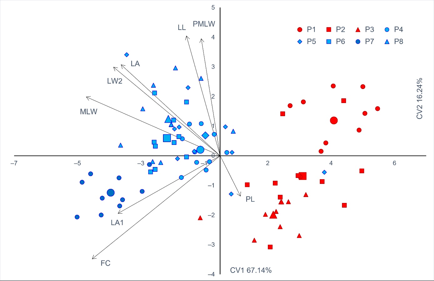
Figure 3. The first two canonical varieties of the canonical discriminant analysis (CV1 and CV2) of eight Salix eleagnos populations based on eight morphological traits. Each individual tree is indicated by a small sign, while the population barycenters are represented by larger ones. The colour of the signs is related to the two groups of populations detected from K-means clustering method (cluster A–red, cluster B–blue). Morphometric traits’ acronyms as in Table 4. Populations as in Table 1.
Slika 3. Prve dvije diskriminantne funkcije kanoničke diskriminantne analize (CV1 i CV2) osam populacija sivkaste vrbe na temelju istraživanih morfoloških svojstava lista. Svaki pojedinačni grm označen je malom oznakom, dok su populacijski baricentri predstavljeni većim. Boja oznaka povezana je s dvije skupine populacija dobivene metodom klasteriranja K-means (grupa A – crvena, skupina B – plava). Akronimi morfoloških svojstava kao u Tablici 4. Populacije kao u Tablici 1.
The overall classification rate on the group level was 93.7%. Individuals from karstic populations were correctly classified in 96.7% of cases, whereas the riparian individuals did so for 92.0% of cases. The lowest percent of correctly classified individuals was observed in the P5 population (70.0%). Individuals from P1, P2, P4, P6 and P7 populations were correctly classified in 100% of cases. Figure 1C shows the barplot with posterior probabilities of classification of each individual into each group from the results of the classification analysis of discrimination.
Multivariate diversity index (MDI) and morphological differentiation
Multivarijatni indeks raznolikosti (MDI) i morfološka diferencijacija
The multivariate diversity index values (MDI), based on nine leaf traits, ranged from 1.154 (P6) to 3.480 (P5), both belonging to the riparian group (Table 1). Kruskal-Wallis test confirmed the differences in the MDI values, by testing among all populations. According to the Wilcoxon rank sum test, the highest MDI values were found in populations that had the lowest percentage of correctly classified individuals in CDA (P5 and P4). In addition, Kruskal-Wallis test proved to be significant when differences between karstic and riparian populations were tested.
Using the AMOVA analysis, significant variability on the intra- and interpopulation levels was confirmed (Table 10). Furthermore, individuals from karstic vs. riparian habitats were clearly distinguished. The highest percentage of the overall variability addressed the diversity within populations, the second highest percentage addressed variability between the habitats (karstic vs. riparian), whereas the lowest percentage was assigned to the variability of populations within the same habitat. AMOVA analysis had additionally showed that riparian populations were significantly more diverse than those found within the karstic habitats.
Table 10. AMOVA analysis for partitioning of total morphological variance of Salix eleagnos populations between habitats (karstic vs. riparian), among populations within habitats and within populations, as well as among and within populations of each habitat.
Tablica 10. Rezultati AMOVA analize za raspodjelu ukupne morfološke varijabilnosti populacija sivkaste vrbe između tipova staništa (krških naspram riječnih), između populacija unutar tipa staništa i unutar populacija, kao i između i unutar populacija svakog tipa staništa.
Isolation by distance (IBD) and environment (IBE)
Izolacija uslijed geografske (IBD) i ekološke udaljenosti (IBE)
A simple Mantel test (Figure 4) identified significant correlations ( r = 0.436, p = 0.0220) between morphological and environmental distances, proving an influence of isolation by environment (IBE) on leaf morphology of rosemary willow populations. Isolation by distance (IBD), however, did not contribute to leaf morphological variability, as proven by the lack of significant correlation between morphological and geographic distances ( r = 0.318, p = 0.0966).
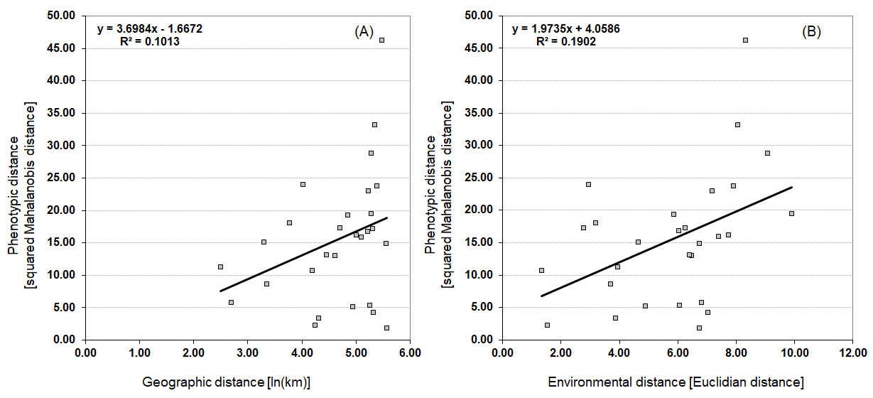
Figure 4. Isolation-by-distance (IBD) and isolation-by-environmental-distance (IBE) in rosemary willow populations. Scatter plots of simple Mantel tests showing the relationships between: (A) geographic and morphological distances ( r = 0.318, p = 0.0966); and (B) environmental and morphological distances ( r = 0.436, p = 0.0220).
Slika 4. Izolacija uslijed geografskih (IBD) i ekoloških udaljenosti (IBE) u istraživanih populacija sivkaste vrbe. Dijagrami jednostavnih Mantelovih testova koji pokazuju odnose između: (A) geografskih i morfoloških udaljenosti (r = 0,318, p = 0,0966); i (B) okolišnih i morfoloških udaljenosti (r = 0,436, p = 0,0220).
RASPRAVA
Rosemary or bitter willow ( Salix eleagnos) is an economically mostly insignificant species (Herman 1971; Schütt 1997), with limited uses for wood, basketry, and biomass, and as such has not been the subject of genetic or morphological research. Therefore, our results could only be compared to older published data in botanical literature. In various flora and textbooks (Herman 1971; Krüssmann 1962; Schütt 1997; Idžojtić 2009), leaves of the species are described as extremely elongated, as confirmed by our research. The size of the leaves, however, has not been extensively reported, and the size ranges from 6-15 cm (Krüssmann 1962; Idžojtić 2009). Mean values revealed by our research are significantly lower, within the 2-3 cm range for karstic populations, and 4-5 cm for riparian populations. The great discrepancy in data is most likely due to the small sample size of the leaves represented in botanical literature. This is a common occurrence, since authors would use a small sample from nature or vouchers from herbariums when writing botanical textbooks or flora, thus being unable to encompass the complete area of research, i.e., the variability of the species.
It is well-known that the levels of genetic and phenotypic diversities and their spatial distribution on population and among-population level, are the result of a mosaic of interactions between intrinsic and extrinsic factors, including phenology, dispersal, topography, and flood regime (Corenblit et al. 2014; Rodríguez-González et al. 2019). In general, our research revealed that karstic populations all had homogeneously low diversity, i.e., they were characterized by similar multivariate diversity index (MDI) low values. This homogeneity is likely the result of smaller populations’ area, as well as the homogeneous habitat conditions in them. In contrast, the riparian populations boasted heterogeneous values of MDI, with some populations being highly diverse, and others having very low MDI values. When riparian populations with low MDI values are considered, they are likely to have experienced a form of genetic drift, i.e., the “founder” effect (Wright 1937; Eckert et al. 1996; Star and Spencer 2013), through which newly formed populations are formed by very small number of individuals and thus boast low diversity levels. This case has been known to happen for willow species (Brunsfeld et al. 1991; Alsos et al. 2015; Tumpa et al. 2022), as well as other pioneer species (Haase 1993; Lowe et al. 2018; Woellner et al. 2021). In theory, a new population of rosemary willow could have grown from seeds of a single individual, which floated downstream. This could have happened in P6 and P7, whose MDI values were lower even than those noted for karstic populations. On the other hand, populations P4 and P5 were found to be highly diverse. These populations are located close to the karstic populations, thus enabling the influx of genes which, when intermixed with the riparian genes, mark them as inherently more diverse. In addition, the heterogeneity of the habitat in these two populations, with numerous plants growing both in the flood zone of the rivers (permanently humid conditions) and on the river terraces (seasonally flooded/above floods), could contributed to the notably higher phenotypic diversity. This is supported by the lowest levels of classification found for P4 and P5 in which, although riparian, some individuals were classified close to karstic populations.
Our analyses indicate that the majority of significant phenotypic variation among individuals occurs within rather than among populations. However, the ANOVA and AMOVA analyses showed that a large part of the total variation could be assigned to the differences between the studied groups of populations, i.e., karstic and riparian. In addition, in the different multivariate analyses carried out under the morphometric material from eight studied populations, we observed two well-differed groups of populations, which coincide with the above-mentioned habitats. Accordingly, small-leaf morphotypes of rosemary willow were found in higher altitude sites, farther away from waterways, and were characterised by higher levels of rainfall, whereas the large-leaf morphotypes were found in riparian sites with lower levels of rainfall. Due to the fact that this species requires a certain level of underground water to thrive (Herman 1971; Schütt 1997), xeromorphic small-leaf morphotypes developed only in sites where ample rainfall could counter the lack of water in soil. Finally, if we assume that the gene flow among populations from those ecologically divergent habitats, karstic and riparian, is reduced because of lower rates of successful establishment of immigrant organisms, which originated in various habitats, as a result of local genetic adaptation (Nosil and Crespi 2004; Noisl et al. 2005, 2008, 2009; Orsini et al. 2013; DeWoody et al. 2015), these two clearly separated groups of populations of rosemary willow could potentially represent two ecotypes – the small-leaf ecotype found in the drier habitats and the large-leaf found in the water habitats. This hypothesis is well-substantiated by the results of the Mantel test and the isolation by environment (IBE) pattern. In other words, we revealed that the ecological distances correlated with morphological distances, i.e., populations from ecologically more similar habitats are also morphologically more similar.
Although all populations significantly followed the environmental gradient, populations within each habitat demonstrated significant differences, i.e., narrow vs. oblong elliptical leaves. According to the AMOVA analysis, these differences are particularly pronounced between populations within riparian habitats. From the riparian populations, P7 stood out by having less elongated leaves when compared to other riparian populations, including population P5, which was located only 20 km away. As previously mentioned, waterways enable movement of plants or genes across the landscape (Rodríguez-González et al. 2019) and are generally known to serve as corridors for riparian plants (Nilsson et al. 2002, 2010; Bothwell et al. 2017). That movement can decrease the genetic difference on one side (Murray et al. 2019), and may influence the spatial distribution of genetic diversity on the other side (Macaya-Sanz et al. 2012), as well as lead to distinctiveness between plant populations. Although most seeds disperse very close to the mother plant, in some cases they can travel farther downstream from the mother plant (de Jager et al. 2019). If the number of individuals that are forming the new populations is small, these populations can phenotypically differ significantly (Nei et al. 1975; Scheepens and Stöcklin 2011). This in particular case, the reason is the weak geographic structure of the populations, as well as the lack of clear isolation by distance (IBD) pattern, in which geographically closer populations would also demonstrate morphological similarities. It has been previously reported that, due to the various factors of influence, drivers of genetic diversity and population structure in riparian plants are not easily discernible (Rodríguez-González et al. 2019). Furthermore, within the arid, karstic population group, P1 stood out by having the most elongated leaves. This population is surrounded by mountain ranges on the western and northern population’s edge, and sea on the southern edge, thus isolating it from other populations. When the effective size of the population is that small, as it is the case in P1, and the population is so isolated, morphological differences are expected (Lesica and Allendorf 1995). The limited gene flow as a result of such isolation usually leads to the creation of specific morphotypes, which has previously been confirmed for a number of plant species (Baker and Dalby 1980; Tremblay 2005; Boratyńska et al. 2005; Galván-Hernández et al. 2020).
Although the southernmost population P8 might have been expected to exhibit extreme differences in leaf morphology, due to its location in Krka canyon and the dual influence of the sub-Mediterranean and continental climate extremes (Perica et al. 2005), this was not the case. Moreover, this population was very similar to the northern populations in river valleys, located 200 km or more away. Our theory is that the specific microclimate in the canyon of this southernmost population managed to mellow down the climate extremes and great oscillations of the daily and annual temperatures so much that the conditions in which the willow grows here are similar to those in the populations farther up north. In this case, we can assume the natural selection and phenotypic plasticity worked in the same direction, i.e., in similar habitats it favoured similar phenotypes (Westoby and Wright 2006; Kimball et al. 2013; Mallet et al. 2014). In addition, it is highly likely that the northern and southern populations in this research belong to the same Last Glacial Maximum (LGM) refugium. Although the northwestern Balkans is considered to be the intermixing zone of different refugia’s lines (Hewitt 1999; Petit et al. 2003), resulting often in differences between the northern and southern populations, for willows this is most likely not the case. In several instances, it has been reported that Salix species, together with other cold tolerant species, i.e., birches, pines, spruces, or larches, were evidently capable of withstanding the LGM at higher latitudes (Willis et al. 2000). We assume that rosemary willow, along with other willow species, was not present in the southern Balkan peninsula during the last glacial period (Huntley and Birks 1983), and that both the northern and the southern populations stem from refugium most likely located in the middle latitudes (Palmé et al. 2003). Palmé et al. (2003) highlight that the light seeds of willows, spread by the wind, had a significant influence on the rapid dispersal of these species during the deglaciations of the Earth. The high dispersal ability of willows could continue to exert influence over its genetic structure, since seed dispersal between populations should prevent population differentiation and cause a wider distribution of the haplotypes. Alternatively, this species is often used as an ornamental plant and the influence of humans on the dispersal of plant material cannot be fully excluded.
ZAKLJUČCI
Our results clearly demonstrate a substantial divergence in phenotypes of rosemary willow when leaves are considered. Leaf phenotypic features displayed a clear bimodal distribution across the populations, with samples from dry karstic habitats having smaller leaves than those from riparian habitats. As expected, the strong phenotypic structure between these two groups of populations was largely explained by the environmental conditions and fits to an IBE pattern. In addition, statistically significant differences were found on both intra- and interpopulation levels. Karstic populations were homogeneously less diverse than the riparian populations, which boasted both the highest and the lowest MDI values noted in the research. This heterogeneity of diversity is the result of specific conditions in which each of the riparian populations is situated, as well as the specific history of inception of the populations (“founder” effect). Overall, our results indicate that the distribution of the phenotypic diversity across rosemary willow populations is strongly related to the environmentally specific factors, probably due to the natural selection and phenotypic plasticity, and stochastic factors such as gene flow, genetic drift and founder events.