
INTRODUCTION
UVOD
Light detection and ranging (LiDAR) technology has been widely used in forestry and natural resource management, particularly forest inventory and management, investigating forest ecology, and road construction (Reutebuch et al. 2005; Singh et al. 2015; Zhao et al.2016; Matinnia et al. 2017; Lou et al. 2023). LiDAR technology enables three-dimensional (3D) point cloud data of objects and the Earth's surface. Also, it can penetrate underneath a canopy of trees. Hence, LiDAR data allows the generation of accurate and precise digital elevation models (DEMs). Precise and accurate DEM generation is crucial in forestry applications, such as extracting canopy height models (CHM) or DEM-derived topographic features (i.e. slope and aspects) (Zhao et al. 2016; Fu et al. 2022; Zhang et al. 2023). Therefore, point filtering to distinguish ground points from non-ground points and generate DEM is the primary and the most critical step in processing raw LiDAR data because it affects the accuracy of generated DEM. LiDAR uses laser pulses. The laser allows us to collect data about objects thanks to the rays reflected from objects on the Earth and their returning. Luo et al. (2023) created a digital elevation model for forest areas using full waveform LiDAR data and hyperspectral image data. Points are classified into different groups depending on surface laser hits. The main group is the first and last return (Dong and Chen 2017). The filtering process was performed assuming that the last return represented the ground (Pingel et al. 2013). Matinnia et al. (2017) produced an accurate and high-resolution digital elevation model from the first and last laser pulses. Chen et al. (2017) created LiDAR by recording the last return points and dividing points into different elevation layers, and obtained digital terrain model by filtering each layer.
With advancing technology, many filtering algorithms have been developed to classify ground points and create DEMs using LiDAR data. While the majority of these filtering algorithms work quite well on flat terrain and sparse vegetation, it is still difficult to filter them in areas with very rugged terrain, steep slopes, dense vegetation, and rugged terrain (Zhao et al. 2016; Cai et al. 2023; Luo et al. 2023). The most important challenge is determining appropriate parameter values for filtering. Yu et al. (2022) applied a ground filter in their proposed algorithm, thanks to the five parameters required by the user. The accuracy of ground filtering algorithms was evaluated and digital terrain models were compared by using the most appropriate parameters in lands with vegetation density and slope (Klápště et al. 2020). The IPTD algorithm was proposed to filter ground points in the forested areas in both topographically and environmentally complex regions. This algorithm was successful in finding steep slopes and peaks thanks to four parameter data (Zhao et al. 2016). Grid resolution, time step, hardness, slope adaptation factor, iteration and classification threshold value parameters were defined for CSF filtering algorithm (Zhang et al. 2016). In this case, finding the right parameters for each terrain type can be time-consuming.
The creation, accuracy, or quality of the DEM impacts usage scenarios (Kraus and Pfeifer 2001; Chen et al. 2017). If a high-resolution DEM is created, the resulting topographic surface and soil subsidence can be easily identified (Matinnia et al. 2017). By using the geometric or radiometric features of LiDAR, the computer's ability to learn from data was also utilized. An improved DBSCAN clustering algorithm is proposed to detect signal photons from ICESat-2 LiDAR data to determine ground elevations in urban areas. By adjusting minPts and eps values in each cluster, ground points were able to be obtained
(Alzaghoul et al. 2021). Machine learning method was used to create landslide hazard map thanks to geomorphological factors derived from DEM (Chang et al. 2019). Deng et al. (2022) proposed an obstacle detection algorithm. With the developed DBSCAN clustering algorithm, an adaptive neighborhood value that changes with distance was determined for each point cloud by the linear interpolation method. Another method based on clustering algorithms was proposed by Feng et al. (2017). With this method, the accuracy when processing boundary points is increased, which revealed its minimum acceptable distance, thus achieving good performance both in terms of accuracy of processing boundary points and time complexity (Feng et al. 2017).
We proposed a new approach for LiDAR ground point extraction in a forested area with dense vegetation. In this approach, firstly, point cloud is divided into appropriate datasets. Three datasets consisting of the last return, the second return and the combination of the first return and the last return were obtained from the airborne LiDAR point cloud data. A grid-based filter was applied to each dataset. Then, machine learning was used in the study. The silhouette value used to determine the number of clusters in the clustering process was this time automatically used to determine the epsilon parameter, and LiDAR ground points were classified. A digital terrain model was obtained with determined ground points and compared with the reference model. When compared to the previous studies, four issues were taken into consideration with the proposed approach. (1) Instead of using the lowest elevation points in the grid- based filtering process, the average elevation value was taken as the threshold value to deal with slope changes. (2) Fast analysis will be possible thanks to a single parameter value entered by the user. (3) For each dataset, the parameter value can be calculated automatically according to the characteristics of the data. (4) It will increase the accuracy of the resulting digital terrain model as more LiDAR ground points are classified after filtering. Additionally, our proposed approach was compared with the CSF algorithm, which is one of the traditional filtering methods. As a result, a highly accurate forest understory topography map can be created with the proposed approach. However, we think it will help decision-making in forestry practices. Additionally, this approach will be tested on other land types and the results will be shared.
MATERIALS AND METHODS
MATERIJALI I METODE
Study area - Područje istraživanja
The area where the study was carried out is the Kirazlı Weir Nature Park within Belgrad Forest in the Eyüpsultan district of Istanbul. The region took its name from the Kirazlı dam built on the Kirazlı stream in 1818. The area is suitable for outdoor activities such as picnics, walking and cycling. In the forest area of the nature park, there is a deciduous forest area including the species such as sessile oak (Quercus petraea), larch (Pinus nigra), shrub (Erica arborea), hornbeam (Carpinus betulus) and complex terrain types. The study area is shown in Figure 1. In addition, measurements were made with total station (TS) to evaluate the accuracy of the model in this region, and 941 ground control points were obtained.
Airborne Laser Systems (ALS) - Zračni laserski sustavi (ALS)
Airborne LiDAR point cloud was created in August 2013 with a Riegl Q680i scanner and a platform mounted on a helicopter, at a frequency of 16 points per square meter.
Approximately 1352010 point data were obtained in the scanning. The surveys were performed in the study region, and the platform height was 600 m. The study area of the nature park amounts to approximately 20 decares. The area where the dam and its surroundings are measured is shown in Figure 2. While ALS is a reliable method for collecting terrain data, creating a high-quality and efficient digital terrain model can be difficult. Therefore, correct classification of points is important for creating a terrain model. For this, less important elements should be removed by data reduction (Liu 2008). Therefore, in our proposed method, data, which can include ground points, are selected from multiple rotations through the data reduction process. Additionally, discrete return LiDAR shows better accuracy in height measurements at individual tree and stand levels (Chen 2007).
Grid-based filter algorithm - Algoritam filtriranja temeljen na mreži
Grid-based filters, one of the surface-based filters, create a reference surface with discriminant functions, after which the point category is determined according to the distance between each point and the corresponding reference surface. Active shape models are used to determine the reference ground surface (Qin et al. 2023). Whether this parameter, defined as cell size or window size, is large or small is important in terms of filtering or reducing the data. Martinez et al. (2019) wanted to identify bridges and water bodies by using LiDAR features such as radiometric and geometric variables. A 2 m x 2 m DEM grid was created and the Z value was determined with the different components created. If the height difference is less than 1 m, these points are considered bridges. Deng L. et al. (2022) used a predefined height threshold value to filter ground points after obtaining a ground surface elevation model. Thus, the size of the data in the dataset was reduced. Du and Wu (2022) calculated the data density by dividing the data field into a limited number of cells with a standard grid structure.
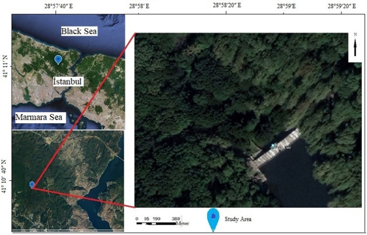
Figure 1. Study area
Slika 1. Područje istraživanja
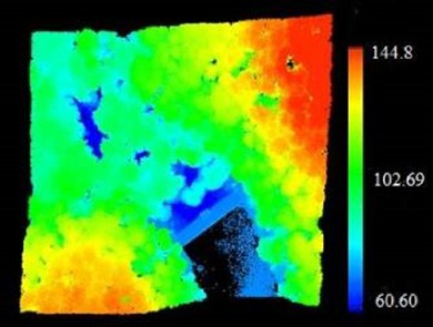
Figure 2. LiDAR data of the study area
Slika 2. LiDAR podaci područja istraživanja
DBSCAN clustering algorithm - DBSCAN algoritam klasteriranja
This algorithm is one of the density-based clustering algorithms, which is one of the spatial data clustering techniques that produces useful models from complex databases, searching for clusters of any size or shapes and identifying outliers. A cluster may consist of a core dataset that is close to each other and a non-core dataset that is close to this dataset (Ester et al. 1996; Schubert et al. 2017). DB- SCAN uses only two parameters that determine whether a region is considered dense enough to belong to a cluster (Gunawan and De Berg 2013). These include: minPts – the minimum number of points clustered together for a region to be considered dense; Eps – the radius of the virtual circle defined separately around each point.
The algorithm randomly checks all points starting from one point in the dataset. If the controlled point has already been included in a cluster, it moves to the next point without taking any action. If the point is not clustered, it finds the neighbor- ing points in the epsilon neighborhood of the point by performing a region query. If the number of neighboring points is more than minPts, it transfers this point and its neighboring points to a new cluster. If there are at least minPts points within the epsilon radius to the point, then it considers all these points to be part of the same set. After that, clusters are expanded by repeating neighborhood cal- culation for each neighboring point. If it has a distance less than epsilon, the point remains inside the cluster. When points are further than epsilon from each other, the point is transferred to a new cluster (Ester et al. 1996; Schubert et al. 2017). Many researchers have tried to find parameter values. Wu et al. (2021) analyzed minPts value with the numbers 2, 4, …, 20 when using clustering algorithm. It
has been confirmed that it can separate data of unequal density into clusters. As a result, it was observed that minPts value had little effect on the clustering results when choosing different values. Zhang et al. (2023) used DBSCAN algorithm to detect trees. Using values eps = 2.15 and minPts = 480, they clustered understory vegetation and low branch leaves well. In addition, when eps = 0.6 and minPts = 3, the lower vegetation was clustered. Thus, although high accuracy analysis was achieved with appropriate parameters, it took time to find these parameters. In our proposed approach, the cluster radius will be determined for the value with the highest eps value and silhouette value within cluster, but minPts value will be determined manually.
Methods
Metode
We present a new approach that classifies ground points to determine topograph- ic features of the terrain using aerial LiDAR data in a densely vegetated forest area. Three separate datasets were obtained from an ALS point cloud: second return, last return and first/last return. Then, Z score algorithm was applied to these three datasets to remove outliers or noise points. Each dataset was then po- sitionally placed in the grid structure. In order not to ignore height differences in the field, a classification was made with average height values of points in a cell. Points below average height value of the points in a cell were classified as possible ground points; otherwise they were classified as non-ground points. Then, clus- tering algorithm was used. Clustering serves as a partitioning task, where objects in same cluster are similar to each other, but other clusters are different from each other. Epsilon value, one of the parameters used in the DBSCAN algorithm, which is one of clustering algorithms, was calculated according to the dataset. Here it was calculated by taking into account height differences of points. The silhouette value, which has verification and interpretation features, was used for this calculation. When the silhouette value was high, epsilon value was automat- ically determined. With this epsilon value obtained, datasets were analyzed with minPts value entered by the user. Thus, they were classified as ground and non- ground points. This proposed approach was performed in Python software. The determined LiDAR ground points were compared with ground control points we obtained. As a result of the analysis, more LiDAR ground points were extracted in a dataset obtained by combining the second return and the last return datasets. Thus, changes in the land surface can be monitored. Additionally, a comparison was made based on the accuracy assessment made with a CSF algorithm, which is one of ground filtering algorithms. In the comparison of LiDAR ground points obtained with the proposed approach and ground control points, mean error, RMSE, kappa and F1 score values, which are vertical accuracy statistics, were cal- culated. As a result, with the approach we proposed, statistical values obtained
by combining the first return, the second return and the last return datasets from LiDAR point cloud showed close accuracies, and similar terrain models were ob- tained in comparison with CSF algorithm.
As the first step in the proposed approach, discrete points were obtained in ALS point cloud. For our approach, they were classified into three datasets: last return, second return, and first/last return. The obtained point count data are shown in Table 1. After all discrete points were determined, noise and outlier points were determined. The number of noise and outliers was 2213. The algorithm was ap- plied for individual datasets. The flow diagram of the proposed approach is shown in Figure 3.
Table 1. The number of return points from ALS datasets
Tablica 1. Broj povratnih točaka iz ALS skupova podataka
|
Second return Drugi povrat |
Last return Posljednji povrat |
First + last return Prvi + posljednji povrat | |
| Points - Točke | 374469 |
13809 |
518396 |
| Min Z | 60.6 |
61.57 |
61.4 |
| Max Z | 129.05 |
124.54 |
144.78 |
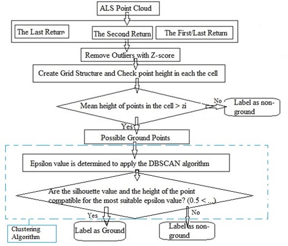
Figure 3. Flow diagram of the proposed approach
Slika 3. Dijagram toka predloženog pristupa
As the second step, Z-score test was applied to each dataset. In this way potential outliers with non-compliant low values in datasets should be removed. Thus, the points that produce both intense noise caused by reflective objects (leaf, water etc.) and less accurate predictions for forest models will be filtered (Gao et al. 2021). The Z-score test is a type of standard deviation that allows us to find the probability of a value occurring in a normal distribution or to compare two samples from different populations (Curtis et al. 2016).
Using the Z-score test, we can find outliers in the desired range and remove them from our dataset. For this, the following equation is used:
Z-score value = (X — μ) / σ (1)
Where X value is our dataset from which we want to calculate the Z-score; μ is the dataset mean; and σ is the standard deviation of the dataset (Curtis et al. 2016).
As the third step, a grid-based filter is applied to LiDAR datasets. Each dataset is transferred to a grid plane according to its spatial values, with a cell size of 3 m x 3 m. Choosing a smaller grid size will increase the number of points in the cell. Additionally, experiments were made by gradually increasing and decreasing cell size, and the most ideal size was selected for each dataset. After placing points on a grid structure, height difference relationship of points in each cell was taken into account. The average height values of points in each cell were calculated as the threshold value. If height value of each point within the cell is higher than the average height value of that cell, the point is classified as a non-ground point in the dataset, otherwise it is classified as a possible ground point. However, slope change on the ground is also taken into account when calculating average height. For example, if there are seven dots in a cell, and the height values of these points are 66, 68, 72, 75, 78, 82, 90, the average height value in this cell is
75.85 when calculated according to Formula 2. Then, points with higher average height values will be removed from this cell and classified as non-ground points. That is, points with height values of 78, 82 and 90 are not ground points. There is a height difference of approximately nine meters at the possible ground points for this cell. In this case, the slope of the ground is also included in the process. If Z is the average height within cell, then the average height value is found according to the procedure in Equation 2.
Z= (2)
Some of points in cell are called boundary points or neighbor points. Since we wanted to obtain ground points in our datasets, if there were points corresponding to the border point or corner point, these points were classified as possible seed points if they were lower than the average height value of points in the cell. Additionally, these points were classified by transferring them to the next neighboring cell. If height of any point of cluster is higher than its neighboring points, any point of cluster should be classified as a non-ground point, otherwise it should be classified as a ground point. In classifying points with clustering and segmentation, the dataset was divided into regular segments and the resulting segments were compared with the neighboring segments in terms of topological and geometric aspects. As long as a ground point is adjacent to some boundary points, the entire ground point can be found by clustering (Deng W. et al. 2022).
As the fourth step, DBSCAN algorithm, one of clustering algorithms, was used. Clusters that would form neighbors to each other in terms of location and geometry were evaluated. To find the epsilon parameter used by the DBSCAN algorithm, a separate value was found for each dataset by taking into account height differences of points. The silhouette index was used to interpret and verify consistency within datasets to be created. Therefore, the highest silhouette value calculated for each dataset obtained was determined as the epsilon value. Silhouette values ranged from -1 to +1, where a high value indicates that object matches well with its own cluster and poorly with
the neighboring clusters. A clustering with an average silhouette width above 0.7 is considered "strong", a value above 0.5 is considered "reasonable", and a value above 0.25 is considered "weak", although this increases with increasing the dimensionality of data. Therefore it may become difficult to reach high values (URL 1). The silhouette value may not perform well if datasets have irregular shapes or are of different sizes (Monshizadeh et al. 2022). In this case, it is important to carefully select the dataset used for analytical methods that are affected by point cloud density, such as vegetation (Petras et al. 2023). Silhouette value can be calculated with any distance measurement, such as Euclidean distance or Manhattan distance. However, our approach is based on height differences. Table 2 shows the values and calculated parameters obtained as a result of applying the proposed approach. After applying the DBSCAN algorithm, outliers were found. These points were classified as non-ground points. The second parameter, minPts, was determined in a smaller number, and it was investigated whether each point was a ground point.
Silhouette value is defined for each sample and consists of two values: a: The average distance between a sample and all other points in the same class; b: The average distance between a sample and all other points in the next closest cluster (Rousseeuw 1987).
Silhouette coefficient for a single sample cluster = (3)
Wu et al. (2021) proposed a method for automatic extraction of rock masses in a 3D point cloud. They used silhouette index to evaluate effectiveness of clustering when applying the K-means algorithm. When a low minPts value was used to cluster datasets with varying densities, HDBSCAN algorithm created smaller clusters in regions with dense data points (Malzer and Baum 2020). Fu et al. (2022) automatically determined trees with the parameter: Eps = 0.72 and minPts = 9. Additionally, if eps value is set too small, the dataset will not cluster in a meaningful way. If eps value is high, it will combine meaningless and meaningful data and place them in the same cluster.
Table 2. Results obtained after the proposed approach
Tablica 2. Rezultati dobiveni nakon primjene predloženog pristupa
RESULTS AND DISCUSSION
REZULTATI I RASPRAVA
Statistical comparison and evaluation metrics - Statistička usporedba i metrika procjene
The point cloud obtained in a forested area with dense vegetation was divided into datasets. The number of ground points obtained in the last return dataset after the application of the proposed approach was the lowest and it is shown in Table 2. It can be seen that the last return will not be considered as ground point. In the clustering stage, silhouette values were calculated as 0.6 for the second return dataset, 0.6 for the last return dataset and 0.5 for the first/last return dataset. These values are within a reasonable or acceptable range. For the second return dataset, silhouette value was calculated as 0.6, eps value was calculated as 0.4, and minPts value was calculated as
5. In the last return dataset, while silhouette value was 0.6, eps value was calculated as
0.6 and minPts value was calculated as 5. In the first/last return dataset, while silhouette value was 0.5, eps value was calculated as 0.1 and minPts value was 15. Since point density was scattered during the clustering stage in this dataset, the most appropriate value was determined as a result of trials. El Yabroudi et al. (2022) stated that minPts value may be small for a dense dataset, but if the dataset is sparse, minPts should be larger. As eps value increases, minPts value will also increase as a larger area is scanned. However, in the first/last return dataset, minPts value (minPts=15) we used for DBSCAN algorithm was chosen higher than in other datasets, and ground points were classified by creating smaller clusters with eps value (eps=0.1). DBSCAN algorithm also has the feature of filtering outliers. After clustering, outliers in datasets were removed from the dataset. This is shown in Table 2. After the three datasets created were filtered with the proposed approach, ground points were determined. The classified LiDAR ground points were compared with 941 ground control points. As a result of the comparison, 445 ground points from the second return dataset, 98 ground points from the last return dataset and 177 ground control points from the first/last return dataset were matched. Statistical values obtained as a result of the proposed approach were calculated. This is shown in Table 3. In addition, as the comparison points from the datasets are different as a result of statistical calculations, statistical results calculated with the combination of datasets obtained are shown in Table 3.
Table 3. Statistical and accuracy values of the data after the proposed approach
Tablica 3. Statističke vrijednosti i točnost podataka nakon primjene predloženog pristupa
More ground control points were obtained in the second/last return and the first/ second/last return datasets. Statistically, average error and RMSE values of the second return and the second/last return datasets are close to each other. Total error, kappa and F1 score values are better than other datasets. As a result of filtering using only the last return dataset, although the average error value and RMSE values seem successful compared to other datasets, total error value, kappa value and F1 score values are unsuccessful. When making measurements in a forest area, it is important not to use the last return dataset alone because the number of laser pulses penetrating vegetation to reach the ground will be inconsistent due to changing density of the canopy level, which will cause irregular ground points and negatively affect the terrain model (Cai et al. 2023). In the first/last return dataset, it is the least successful value according to the average error value and RMSE values. Moreover, although its kappa value showed an acceptable success with 66.33%, it failed with an F1 score value of 0.31. As a result of the statistical result obtained by combining all datasets, ground control point was obtained more times than others. While total error and kappa value were successful, F1 score value was reasonably accurate with 0.49. To evaluate analysis results of data, total error, and kappa and F1 score values were calculated according to Table 4.
Table 4. Filtered result comparison matrix
Tablica 4. Matrica usporedbe filtriranih rezultata
|
Filtered results Filtrirani rezultati | |||
|
Ground points Terenske točke |
Non-ground points Ostale točke | ||
|
Reference Referenca |
Ground points Terenske točke |
a | b |
|
Ostale točke |
c | d | |
Toplam Error = (b + c) / (a + b + c + d) (3)
Kappa = 2 x (a x d – b x c) / (a + c) x (c x d) + (a + b) x (b x d) (4)
F1 Score = 2 x a / (2 x a + c + b) (5)
Kappa value indicates the ratio of correct predictions made in system to all predictions. In this case, it determines the overall performance of the model at a reasonable level. The F1 score value does not make an incorrect model selection in unevenly distributed datasets. It also evaluates performance of the model in terms of both accuracy and sensitivity. When evaluating accuracy, it is more logical to do it based on datasets (URL 2).
Finally, ALS point cloud was classified with the CSF ground algorithm using parameters of 0.3 grid resolution, 500 iterations and 0.5 classification threshold. As a result of classification, an average error value of 19 cm and RMSE of 0.213 were calculated. It was successful compared to RMSE and average error values of other datasets. However, while kappa value provided a success rate of 83.12%, F1 score value showed reasonable success with 0.45. The terrain model created from values obtained with total station (TS) and CSF algorithm is shown in Figure 3. A terrain model of these obtained values was created, which is shown in Figure 2. Here, high data volume and method selection were important.
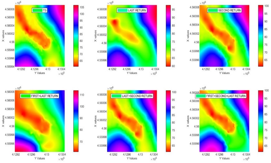
Figure 4. Terrain models created with TS with all datasets
Slika 4. Modeli terena stvoreni pomoću TS-a sa svim skupovima podataka
Additionally, there was a ground point that our proposed approach misclassified based on accuracy evaluation. To understand this situation, we filtered each of the datasets classified as non-ground points again in Table 2. The results obtained are shown in Table 2. The number of points found out of the existing 941 ground control points included: 15 ground control points in the second return dataset, 8 in the last return dataset, and 27 ground control points in the first/last return dataset. Since there were misclassified ground points, more LiDAR ground points could be obtained thanks to the proposed approach by increasing the experimentally determined cell size. In addition, 64 ground points were obtained from non-ground points made with the CSF algorithm. The model made with a total station was chosen as the reference model and was obtained with Matlab software.
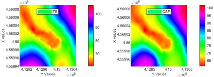
Figure 5. TS and CSF terrain models
Slika 5. TS i CSF modeli terena
Even though they were successful according to RMSE values with the last return dataset compared to the reference land model, both accuracy values were not similar to the model and they were unsuccessful. Differences were obvious when comparing the first/ last return dataset with the reference model. The similarity with the reference model was high in the second return dataset and the second/last return dataset. There were differences in 68-75 m altitude range for the first/second/last return dataset. CSF terrain model, on the other hand, was more similar to the terrain model obtained from the first/ second/last return dataset.
CONCLUSIONS
ZAKLJUČCI
It was aimed to extract ground points using aerial LiDAR data in a deciduous forest area with a complex terrain type. Both surface-based filter and machine learning methods were used. Position and height values of the points were used with grid- based filtering. Machine learning, on the other hand, helped us to either classify data according to developed models or make predictions for future outcomes based on the models. Although learning-based methods perform well in identifying key points, they can cause incomprehensible misclassifications in some cases (Qin et al. 2023). Correct datasets must be selected to prevent misclassification and loss of time. The method we applied for the last return, the second return and the first/last return datasets was the result obtained by combining the second/last turn analysis of ideal data in a forest area with a complex structure for place points. Moreover, this approach can be developed further. Thanks to the proposed approach, extracting more LiDAR ground points in densely vegetated forest areas can help the following activities: 1) it can help assess fire risks in forest areas through analysis of factors such as tree density, height and slope; 2) it can create water flow patterns and assess erosion risks; 3) it can help with road and infrastructure planning in forest areas; 4) it can create a forest inventory thanks to correctly classified above-ground points; 5) if the study area is a deciduous forest, it can be important in mapping different habitat types and biodiversity by obtaining information in terms of both tree species, plant species and animal species.