
Key words: classification, WorldClim, maximum entropy, modelling and mapping, species distribution INTRODUCTION
UVOD
A healthy forest ecosystem possesses a complex and dynamic structure, supporting a rich diversity of plant and animal species (Ürkmez and Gülsoy, 2023; Tekeş, 2024). For a forest ecosystem to be considered healthy, it should effectively fulfil its economic, ecological, and sociocultural functions (Bengston, 1994; Chiesura and De Groot, 2003; Aznar-Sánchez et al., 2018). From an ecological perspective, one of the key functions of forests is the presence of certain wildlife species (classified as keystone, flagship, and indicator species), serving as a marker of a healthy forest ecosystem (Özçelik, 2006; Tekeş and Özkan, 2024). However, even in tropical regions, often regarded as examples of healthy forest ecosystems, forest areas are being lost at an alarming rate of approximately 0.8% per year, with about 10% destroyed over the past 25 years due to human activities (Bradshaw et al., 2009; Arora, 2018). Such forest destruction leads to serious issues, including shrinking, fragmentation, and even complete loss of wild animal habitats.
Ensuring a healthy habitat integrity for wildlife is a priority for sustainable wildlife ecology and management. Therefore, in the geographies where a wildlife species is distributed, four habitat factors including cover, food, water and space must be present at the same time and in the required amount (Selmi, 1985; Evcin, 2022). The decrease or loss of function of any of these four habitat factors causes the habitat integrity to deteriorate (Negiz and Erfidan, 2024; Dogan et al., 2025; Tekeş and Özkan, 2025). Today, although there are many biotic and abiotic factors in the disruption of wildlife habitat balance, one of the biggest factors is the changing climate conditions on a global scale (Evcin et al., 2019; Evcin, 2023). In fact, as climate change profoundly affects the structure and functioning of forest ecosystems (Tekeş vd., 2024a; Tekeş vd., 2024b), wild animal species have also taken their share from this situation.
The Intergovernmental Panel on Climate Change (IPCC) was established in 1988 to protect biodiversity resources against changing climate conditions or to ensure that they are overcome with minimal damage (IPCC, 2024). Thanks to the conferences held by the IPCC, global climate models have been brought to the forefront between different years. The global climate models put forward have three main bases: scientific basis, adaptation studies and prevention measures (Agrawala, 1998; Magnan et al., 2022; IPCC, 2024). Within the framework of these approaches, scenarios created for climate models are used to take the necessary precautions for target species and to reveal their current and future distribution (Sinclair et al., 2010; Evcin and Kalleci, 2020). In this context, species distribution modelling (SDMs) methods come to the fore to reveal habitat suitability for the present and the future (Özkan, 2012).
Species distribution models have recently become popular for assessing the impact of climate change on species, prioritizing conservation measures, or studying invasive species distribution (Kıraç and Mert, 2019; Dilbe et al., 2022). Species distribution models typically link known species distributions with environmental variables, allowing for the prediction of their potential distribution across other regions and over time. One of the species distribution modelling methods is the maximum entropy software. The MaxEnt method stands out by providing the most accurate and reliable results with the least amount of data for wild animal species. The main purpose of the MaxEnt method is to explain that the variable is limited to limited ranges, that is, arbitrarily limited, and the measure of the uncertainty of this variable. Moreover, the MaxEnt method is important in simulating the distribution of animal species with limited distribution areas under changing climatic conditions on a global scale (Dudik et al., 2004; Phillips et al., 2006; Baldwin, 2009; Elith et al., 2011; Hayat et al., 2024).
Chamois (Rupicapra spp.) is naturally distributed in the mountainous regions of Europe and West Asia (Corlatti et al. 2011), and, according to the International Union for the Conservation of Nature (IUCN) category, the species is stated to be of Least Concern (LC) and under protection based on the number of individuals (IUCN, 2024). Despite the systematic implementation of chamois conservation and management plans, at local (population) level, it is reported that changing climatic conditions will cause the habitats preferred by the species to have a localized form (Huş, 1953; Başkaya, 2000).
In the light of the information above, this study aimed to map the displacement of the chamois habitats in Europe because of global climate change, viewed as a precursor to the possible destruction of natural ecosystems. For this purpose, the maximum entropy method was used for mapping the actual and potential habitat suitability of the chamois according to different WorldClim climate scenarios (HadGEM3-GC31-LL/SSP126-SSP245-SSP585) for the future (2100) and the current (2010) year. As a result, these maps were classified as very suitable, suitable and unsuitable areas for the habitats preferred by the species and were compared with each other. Thus, it was revealed whether global climate change is a threat for the chamois.
MATERIJALI I METODE
Study area and chamois data collection - Područje istraživanja i prikupljanje podataka o divokozama
Chamois is considered the most widely distributed mountain ungulate wild mammal in Europe and the Near East (Corlatti et al., 2011; Kati et al., 2020; Lovari et al., 2020). However, despite its wide distribution area in the world, there are regional or small-scale studies that reveal the effects of global climate change on chamois (Ciach and Peksa, 2018; Lovari et al., 2020; Chirichella et al., 2021; Anderwald et al., 2024). In addition, no modelling or mapping study has been found among these studies to reveal the effects of climate change on the chamois in Europe. Therefore, to fill this gap in the literature, Europe was chosen as the study area to reveal whether climate change poses a threat to the chamois (Figure 1).
To fill the gap in modelling and mapping of climate change and to improve the existing knowledge about the chamois distributed in Europe, which was determined as the study area, presence data of the target species were obtained from the Global Biodiversity Information Facility (GBIF) data infrastructure (GBIF, 2024). For the chamois, 129 894 presence data were obtained from the GBIF database. The obtained presence data were classified according to the inventory method and 13 138 presence data were taken as a basis for the current and future habitat suitability modelling of the species. Information on the spatial distribution of 13 138 presence data belonging to the chamois within the study area is shown in yellow on the map (Figure 1).
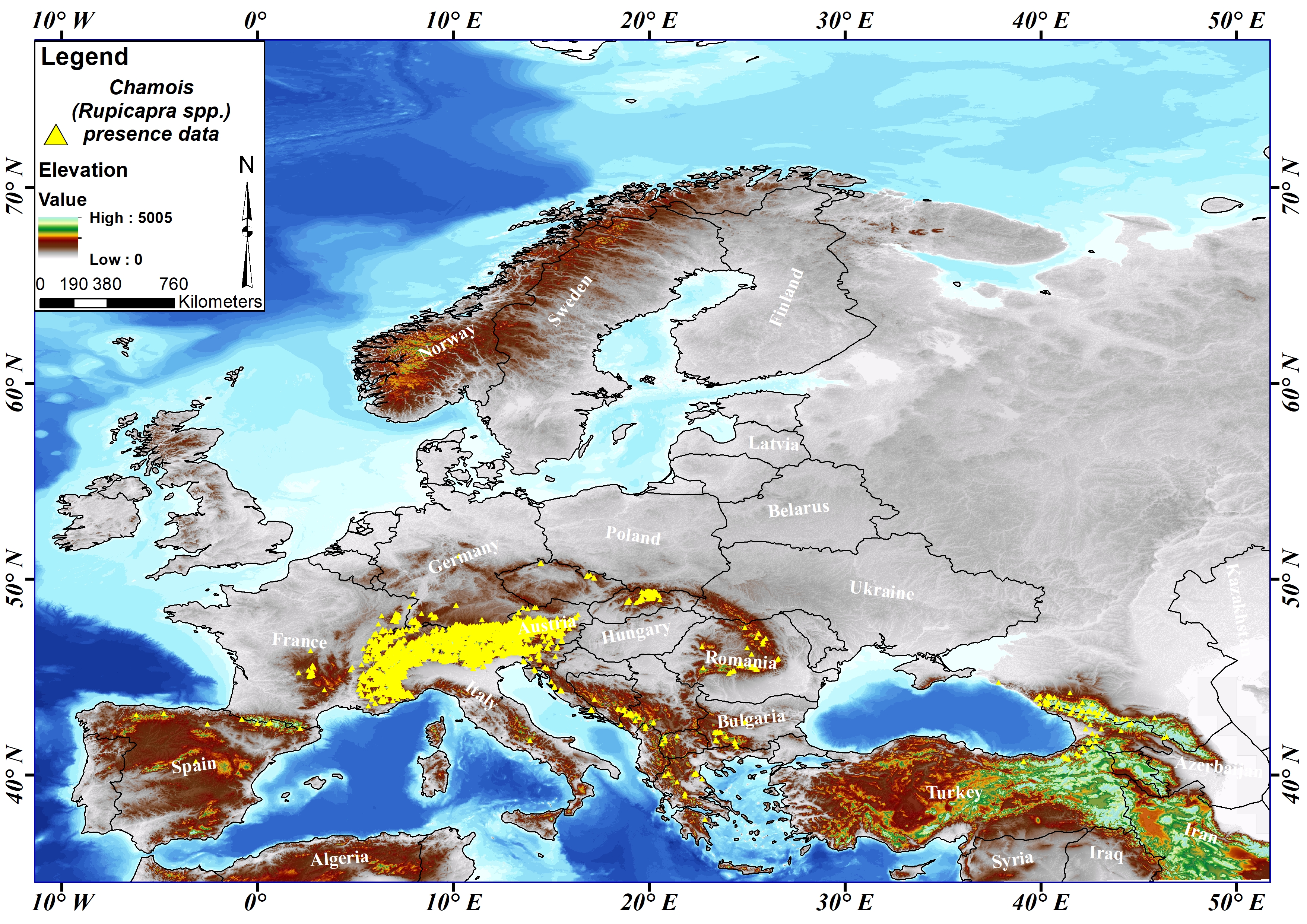
Slika 1. Prostorna distribucija podataka o prisutnosti divokoza (13 138) diljem Europe
Creation of environmental and climatic (WorldClim) data - Kreiranje podataka o okolišu i klimi (WorldClim)
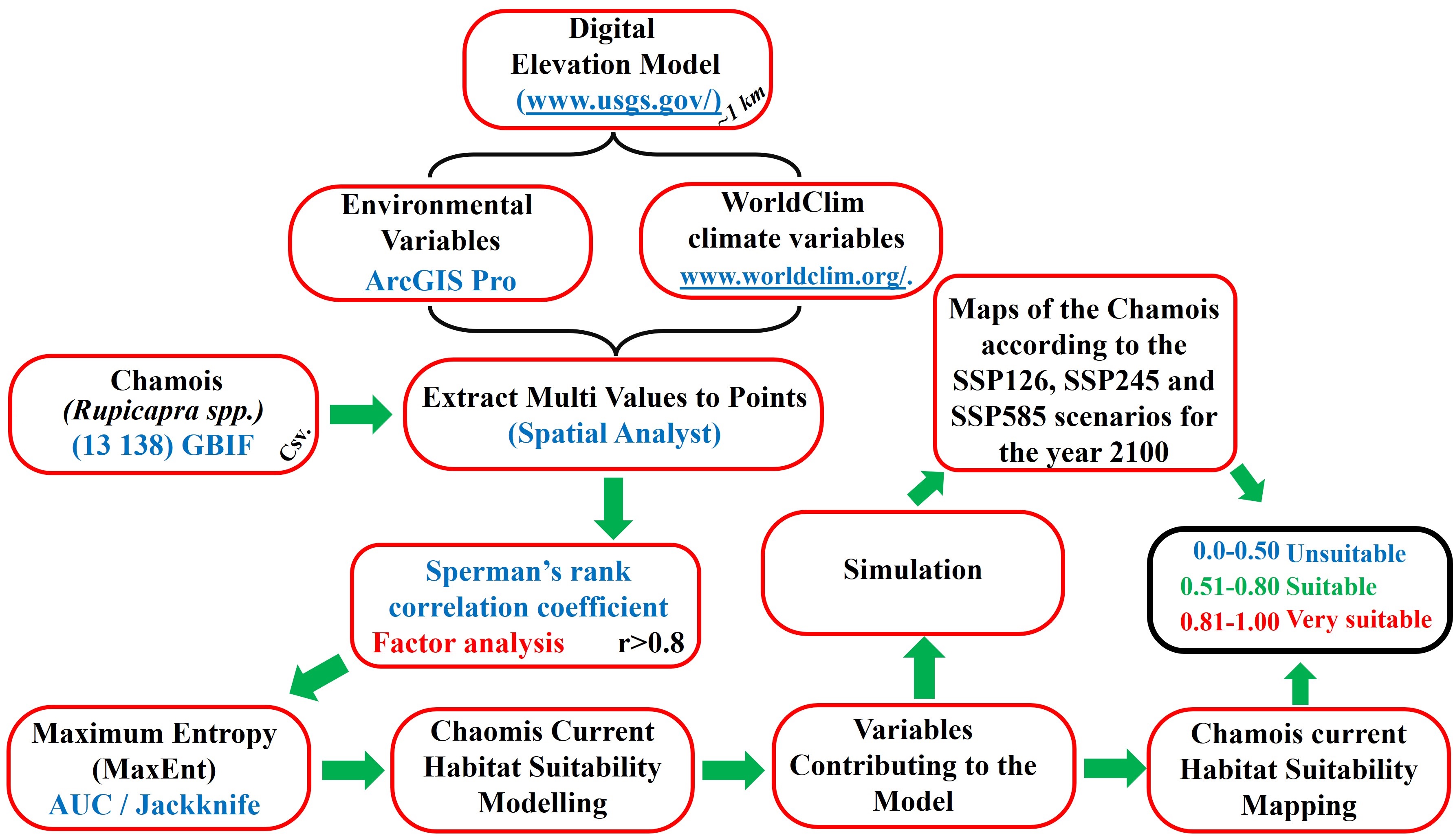
In order to reveal the effects of the predicted global climate change on the chamois in the Eurasia, firstly a high resolution (30 arc seconds, ~1 km) digital elevation model of the study area was obtained from US Geological Survey, USGS (https://www.usgs.gov/) in the GCS_WGS_1984 coordinate system. Base maps of various topographic features of the study area were prepared. Some of these base maps were produced with elements such as aspect, aspect classes, slope, slope classes, landform classification, terrain ruggedness index, roughness index and topographic position index. In addition, base maps of slope length and steepness factor (LS-factor) index, hill shade index, compound topographic index, heat load index, solar radiation index and solar illumination index at different hours (6am/8am/10am/noon/ 2pm/4pm/6pm/8pm/solar illum) were produced (McCool et al., 1997; Keating et al., 2007; Gaughan et al., 2008; De Reu et al., 2013; Momm et al., 2013, Mokarram et al., 2015; Shaver et al., 2019; Habib, 2021).
In studies conducted to reveal the effects of global climate change on the habitats where wildlife target species are distributed, WorldClim or CHELSA climate variables are preferred. Although CHELSA climate variables were introduced in 2017, WorldClim climate variables were updated again in 2022 (Karger et al., 2017; Fick and Hijmans, 2017; Cerasoli et al., 2022). Therefore, WorldClim climate data are the most up-to-date among global climate variables (https://www.worldclim.org/). WorldClim climate data is available on the internet at different scales: 10 minutes, 5 minutes, 2.5 minutes, and 30 seconds. In this study, base maps with a pixel value of 30 arc seconds ~1 km were preferred to have the same resolution as the environmental variables produced. WorldClim climate data includes 19 different numerical climate variables, from bio1 to bio19, for current and future (2040/2060/2080/2100) years. Numerical climate variables include different climate envelope models depending on precipitation and temperature values. One of these climate models available on a global scale, HadGEM3-GC31-LL model, was used to obtain digital base maps for different scenarios SSP126-SSP245-SSP585 for current and future (2100) years. As a result, after determining the variables contributing to the chamois current habitat suitability model, different scenarios (SSP126-SSP245-SSP585) for the year 2100 were simulated.
Statistical analysis - Statistička analiza
The statistical analysis phase was conducted to determine whether there was a relationship between the independent variables obtained from the maps of the independent environmental and climatic variables produced with the chamois presence data which have suitable coordinates as the dependent variable. The similarity of the values of the independent variables causes the variables to show high correlation with each other. This high correlation reveals the multicollinearity problem, which makes it difficult to understand and interpret the relationships between dependent variables and independent variables. In addition, the reliability of the models created for the wild animal species decreases and the results can be misleading. To eliminate this problem, Spearman’s correlation analysis was applied to the independent variables in the RStudio program, and because of the analysis, the variables with high correlations were eliminated. Therefore, to prevent the problems mentioned above, factor analysis was applied to climate variables among themselves in the SPSS program and the best representative variables on chamois distribution were determined (Joliffe and Morgan, 1992; Hauke and Kossowski, 2011). After these processes, modelling studies of the chamois were started.
Maximum entropy (MaxEnt) - Maksimalna entropija (MaxEnt)
The modelling approach based on maximum entropy theory is an effective technique used to reveal species distribution. This modelling technique, which is based only on species presence data, can estimate potential areas that are suitable or not suitable for the distribution of species using the variables of the point where the presence data is taken. The maximum entropy (MaxEnt) method makes area estimates with randomly generated background points using the probability of species existence. The MaxEnt technique performs a two-stage calculation to be able to make estimates and reveal species distributions. First, it calculates density using the variables in the areas where the species is present, after which it calculates the density of points where the species can potentially be found using the variables in the entire area (Phillips, 2005; Elith et al., 2011). As a result of the calculations, estimated values varying between 0 and 1 are created for all points in the study area, and a potential distribution model and map emerges according to these values.
In selecting the correct and valid model, the area under curve (AUC) curves of the training and test data sets should be examined first. The AUC value is between 0.5 and 1, and as this value approaches 1, the success of the model increases. The model AUC values made with the MaxEnt method were classified according to Baldwin (2009) as “very good” if AUC≥0.9, “good” if 0.7<AUC<0.89, and “uninformative” if AUC<0.69. It is also emphasized that the test data set AUC value presented for the model cannot exceed the training data set value. Finally, within the scope of AUC, the training data set AUC value is expected to be the highest and the difference between this value and the test data set AUC value is expected to be low. Another method for checking the degree of accuracy is to examine the jackknife graph of the variables contributing to the model. According to this graph, care should be taken to ensure that the contribution value of any of the variables contributing to the model does not exceed the contribution value to the entire model. In addition, the modelling process should be continued until at least two variables remain that contribute to the model. The workflow diagram for this study conducted in this context is shown below (Figure 2).
Slika 2. Dijagram toka studije
Variable selection - Izbor varijabli
Prior to conducting habitat suitability modelling for the chamois, literature studies indicated a strong correlation between global climate variables (Süel et al., Özdemir et al., 2020; Acarer, 2024a; Acarer 2024b; Özdemir, 2024; Şentürk, 2024). In this respect, the correlation between 19 different climate variables created with high resolution throughout Europe was examined. According to the correlation analysis results presented using the RStudio program, it was determined that there is a high correlation between WorldClim climate variables (Figure 3). When the results of this high correlation were compared with literature studies, the same situation was encountered.

Slika 3. Rezultati Spearmanove analize korelacije ranga primijenjeni na 19 klimatskih podataka
After determining the bioclimate variables that show high correlation with each other, it is necessary to determine the effective climate variables on the chamois distribution. In this context, the Factor Analysis option of the Dimension Reduction plugin in IBM SPSS software was applied to 19 different bioclimate variables. According to the Factor Analysis results, it was determined that the model of 3 variables was 89.927% cumulative and 13.537% of variance (Table 1). Based on this, it was determined that the variables that would best represent the chamois distribution were annual precipitation (bio12: 0.925), temperature seasonality (bio4: 0.671) and temperature annual range (bio7: 0.757) according to their component values (Table 2).
Table 1. Factor analysis results applied to WorldClim variables
Tablica 1. Rezultati faktorske analize primijenjeni na varijable WorldClim
| Total Variance Explained | |||
| Component | Extraction Sums of Squared Loadings | ||
| Total | % of Variance | Cumulative % | |
| 1 | 11.042 | 58.115 | 58.115 |
| 2 | 3.472 | 18.275 | 76.390 |
| 3 | 2.572 | 13.537 | 89.927 |
Table 2. Component matrix results (r2) applied to Chelsa bioclimate variables
Tablica 2. Rezultati matrice komponenti (r2) primijenjeni na varijable bioklime Chelsa
For the chamois habitat suitability modelling, the MaxEnt method version 3.4.4 was preferred. Statistical analysis was applied to 41 different (22 environmental and 19 climate variable) base maps produced at the beginning of the study. According to the results of the applied statistical analysis, modelling processes were performed on 25 base maps, 22 environmental and 3 climate variables. According to the MaxEnt procedure, the maps were converted to the ASCII format. The modelling phase was started with 13 138 presence data and 25 different base maps belonging to the chamois.
Chamois (Rupicapra spp.) habitat suitability modelling and mapping - Modeliranje i mapiranje prikladnosti staništa divokoze (Rupicapra spp.)
While modelling, 10% of the presence data obtained for the target species were randomly divided into 10 replications as test data. Thus, the model processed 13 138 presence data obtained for the target species, 1 314 data were tested, and 11 824 presence data were processed as training data. Cross validation option and 5000 iteration options were preferred for separated presence data. Thus, an average model was created by using all presence data obtained for the target species.
REZULTATI I RASPRAVA
Chamois current model and map - Model i karta trenutne rasprostranjenosti divokoze
A total of 43 different models were created with 25 different numerical base variables for the chamois current habitat suitability model. The elimination process among the variables contributing to the formation of the models continued by removing the variable that contributed the least to the formation of the model. Thus, the modelling process continued until at least two contributing variables remained. The obtained models were first evaluated according to the training test data set AUC and test data set AUC values. Among the presented models, it was determined that the training data set AUC value was 0.839 and the test data set AUC value was 0.834 (Figure 4A). In addition, it was determined that the average AUC value of the model was 0.839 and its standard deviation was 0.004 (Figure 4B). When the AUC values of the detected model were evaluated according to the classification determined by Baldwin (2009), it was determined that it was in the “good” model category. According to the jackknife chart, it was determined that the variables contributing to current chamois model, which is in the good category, are ruggedness, elevation, annual precipitation (bio_12) and temperature annual range (bio_7) (Figure 4C).
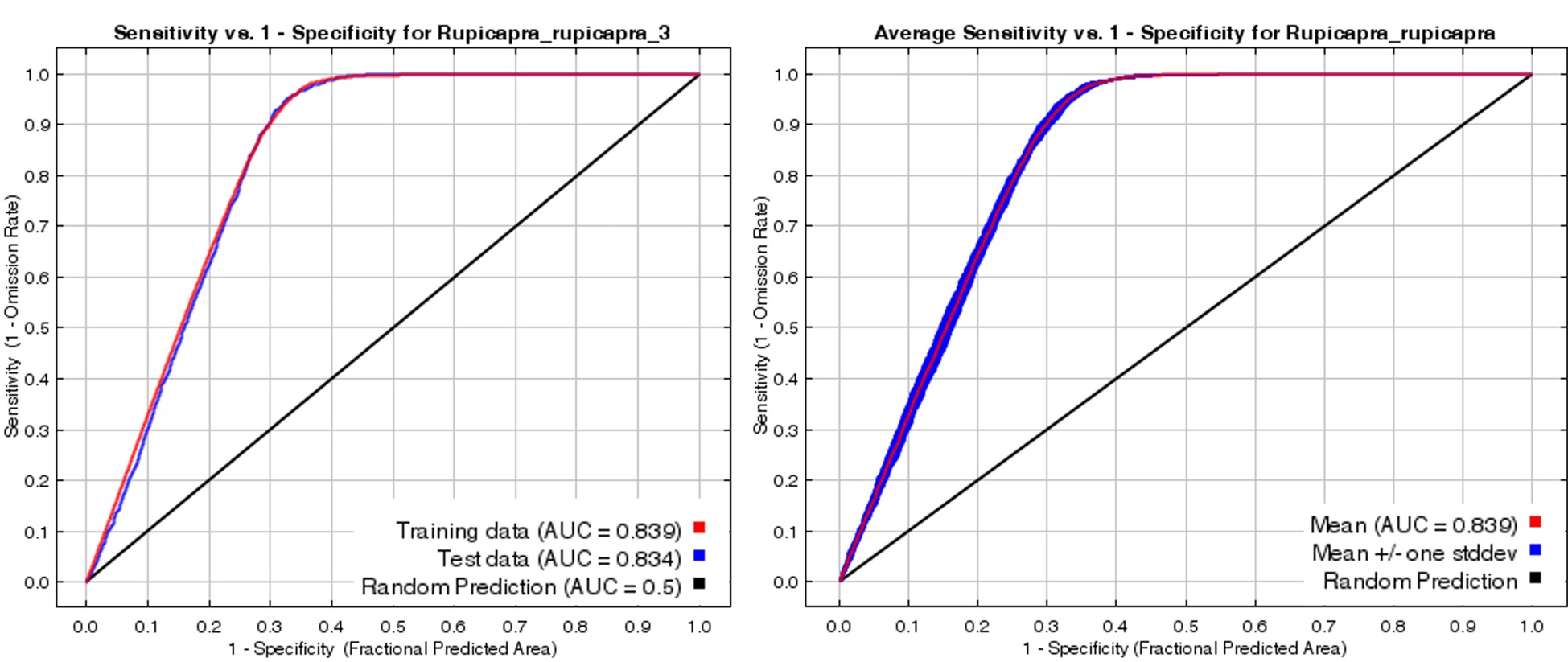

Figure 4. Chamois current habitat suitability model A) training and test data set AUC, B) average AUC and C) jackknife graph
Slika 4. Model prikladnosti trenutnog staništa divokoze A) AUC set podataka za treniranje i ispitivanje, B) prosječni AUC i C) jackknife grafikon
Marginal responder curve graphs of the variables contributing to the jackknife graph of the chamois current habitat suitability model need to be examined. According to the ruggedness variable that contributes the most to the model, it was determined that the probability of the species existing is higher as the ruggedness value within the area increases (Figure 5A). It ensures higher survival rate for ungulates (Gaillard et al., 1998; Edelhoff et al., 2023), since animals use the type of terrain as a proxy for potential escape (Sappington et al., 2007) and associated with this it is one of the ecological drivers of chamois population size (Chirichella et al., 2015). However, from the management point of view on the rugged terrains it is very difficult to estimate population parameters of the mountain ungulates (Wingard et al., 2011).
The elevation variable contributing to the model indicated that chamois distribution is the highest between 1500 and 2500 meters. Although there is a possibility of existence in areas lower or higher than these values, it seems that it mostly prefers lower over higher elevations (Figure 5B). In the cold season, chamois move from 1900-2200 m above sea level and in the hot season, from 2100-2600 m above sea level. It was reported that they mate at high altitudes in the summer (Nesti et al., 2010; Von Hardenberg et al. 2000). However, the snowfall that starts in the cold season carries the estruses female chamois to lower elevation (Lovari et al. 2006).
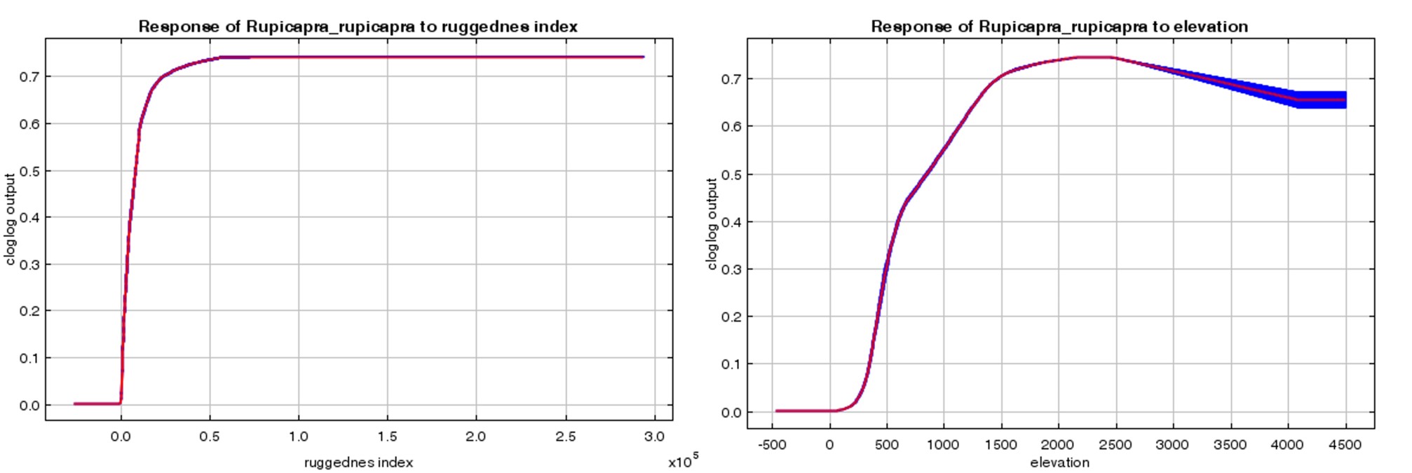
Slika 5. Doprinos trenutnom modelu prikladnosti staništa divokoze: A) indeks otpornosti i B) grafikon nadmorske visine
When the annual precipitation variable contributing to the model was examined, areas where the annual precipitation within Europe was between 600-1600 mm were determined as suitable areas for chamois distribution (Figure 6A). Heavy winter precipitation has significant effect on chamois population dynamics (Donini et al., 2021), and where annual rainfall in the region varies between 700-1200 mm and there is a negative correlation between the increase (Brivio et al., 2016) in annual precipitation and the daily activities of the chamois, thus providing evidence on seasonal distribution and habitat preferences. In this context, it was found that the annual precipitation of the study area was approximately 1200 mm, and the precipitation amount was effective on the chamois distribution (Papaioannou et al., 2015).
According to the temperature annual range variable, which contributes the least to the current chamois habitat suitability model, areas where the temperature value within the area is between 21-26°C were determined as areas where the distribution of the species is high (Figure 6B). They were determined as the best habitat for the chamois. It was found that temperature affects the daily activity and habitat preference of the target species (Von Elsner-Schack, 1985), and that extreme temperature increases negatively affect body mass (Rughetti and Festa-Bianchet, 2012), emphasizing that global warming may be a very real threat to the long-term survival of the chamois population (Papaioannou et al., 2015). As a result, the annual precipitation variable contributing to the chamois current habitat suitability model is in the same direction as the literature. However, although temperature is generally effective in species distribution, no study has been found that provides information about the temperature annual range variable. Therefore, the temperature annual range variable value results of this study will contribute to the literature.
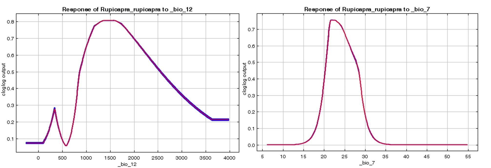
Slika 6. Doprinos trenutnom modelu prikladnosti staništa divokoze: A) grafikon godišnjih padalina (bio_12) i B) godišnjeg raspona temperature (bio_7)
Based on the variable values contributing to the model, the chamois habitat suitability map predicted by the MaxEnt method was presented (Figure 7A). When this mapping of the current model was examined, it was determined that the habitat suitability of the chamois distribution was high in Central Europe and the Balkans. In addition, although the high and rugged parts of the region called the Scandinavian Mountains between the borders of Sweden and Norway were determined as suitable areas for chamois distribution, it was determined that this suitability had a lower value compared to Central Europe and the Caucasus. In this context, this habitat suitability map obtained was classified into unsuitable, suitable and very suitable areas (Figure 7B). According to this classification for chamois distribution, it was determined that 72.29% of the study area was unsuitable, 16.21% was suitable and 11.50% was very suitable.

Slika 7. Sadašnja prikladnost staništa divokoze: A) mapiranje i B) klasifikacija
Chamois future map
Future mapping 1 (SSP126 scenario)
These variables (bio7 and bio12) were converted to the working format of the MaxEnt method in the SSP126-SSP245-SSP585 climate envelope models for the HadGEM3-GC31-LL scenario of the year 2100. In this context, the simulation process was started based on the recent chamois habitat suitability model. The simulation process was first applied to the SSP126 envelope model for the year 2100 and mapped (Figure 8A). When the mapping of this SSP126 envelope model was compared with the present-day chamois habitat suitability mapping, chamois habitat suitability was again found to be higher in the Scandinavian Mountains. However, in the Caucasus and Türkiye, this suitability was found to be lower than the present habitat suitability map. Similarly, this habitat suitability map was classified as very suitable, suitable and unsuitable (Figure 8B). According to this classification, it was determined that 75.29% of the study area for future chamois distribution was unsuitable, 14.73% was suitable and 9.98% was very suitable.

Slika 8. SPP126 scenarij prikladnosti staništa divokoze u godini 2100. A) mapiranje i B) klasifikacija
Future mapping 2 (SSP245 scenario)
After the future mapping of the chamois SSP126 scenario was presented, the SSP245 scenario was analysed. The processes carried out for the SSP126 simulation were applied to the SSP245 scenario. In this context, the chamois habitat suitability map was presented according to the SSP245 scenario for the year 2100 (Figure 9A). When this mapping was examined, it was determined that the suitable areas for the species clearly decreased from the southern part of the study area to the northern part. According to this map classified in the same way, it was determined that 78.47% of the study area were unsuitable, 13.68% were suitable and 7.85% were very suitable (Figure 9B).

Slika 9. SPP245 scenarij prikladnosti staništa divokoze u godini 2100. A) mapiranje i B) klasifikacija
Future mapping 3 (SSP585 scenario)
Finally, chamois habitat suitability was simulated and mapped for the 2100 SSP585 scenario (Figure 10A). According to this mapping, it was determined that the very suitable areas for chamois in the Balkans and Turkey would be destroyed. In this context, it was determined that the very suitable areas would remain only in Central Europe and the Scandinavian Mountains, and that these areas were limited. This map was divided according to habitat suitability classification values (Figure 10B), it was determined that 83.79% of the study area was unsuitable, 13.34% was suitable, and 2.87% was very suitable.
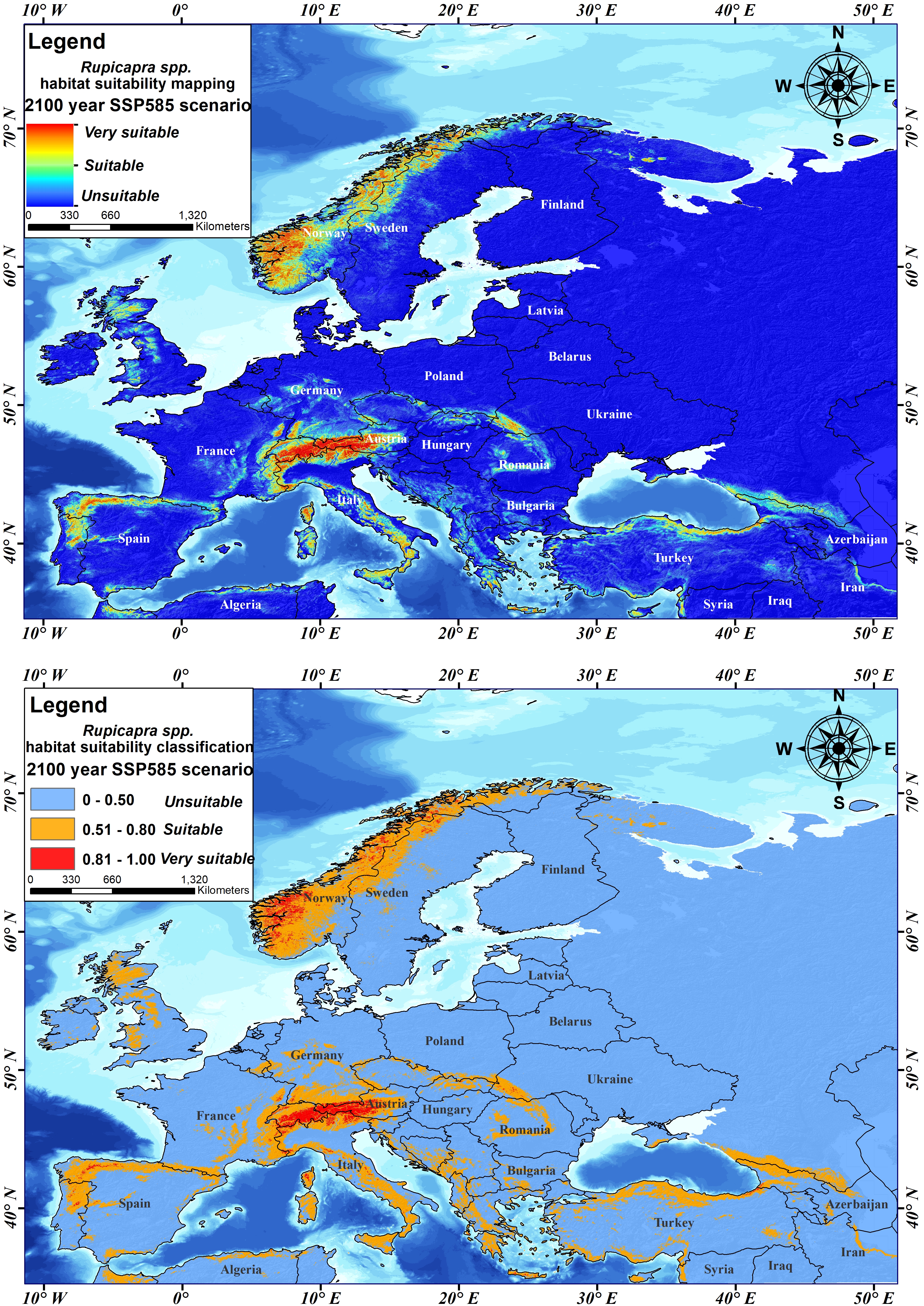
Slika 10. SPP585 scenarij prikladnosti staništa divokoze u godini 2100. A) mapiranje i B) klasifikacija
The effective variables on the chamois distribution, which has a wide distribution around the world, are ruggedness, elevation, annual precipitation and temperature annual range. According to the values of these variables, the maps predicted by MaxEnt according to the present year and the year 2100 (SPP126, SSP245 and SSP585) sequences of the chamois type have been revealed. According to the classification, it was determined that chamois prefers a total of 27.71% of the recent distribution area, 24.71% according to SPP126 scenario, 21.53% according to SPP245 scenario and 16.21% according to SPP585 scenario (Table 3). Therefore, chamois current habitat use rate decreases by approximately 42% compared to the SSP585 scenario for the year 2100. Consequently, global climate change is a threat, not a change, to the chamois distribution.
ZAKLJUČCI
This study offers a valuable understanding of how climate scenarios associated with global change pose a significant threat. Habitat classification indicates that chamois habitat preferences will shift, irrespective of which scenario unfolds in the 21st century. Proactive management is urgently required to reduce these pressures anticipated by global climate models. If adequate protection, management and planning studies are not carried out, chamois will not only be displaced, but the species will become endangered. If this situation continues, wild animals’ extinction will be unstoppable. Wildlife managers are encouraged to evaluate these findings, which raise significant alarms about global climate change and species displacement in order to overcome it with minimal damage.