
INTRODUCTION
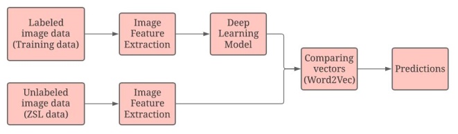
In this day and age, even as we are collecting a lot of data in various fields, there are some categories where it is difficult to collect relevant data. In these particular categories, the mechanism of zero-shot learning (ZSL) can be used to perform classification tasks for unknown object categories that have not been used for training the model. Traditional machine learning approaches mainly focus on predicting data of only the categories they have been trained on. ZSL instead focuses on classifying data of new and unseen categories. This approach can be used in various applications ranging from autonomous vehicles to healthcare use cases. Unseen food dishes are classified and recognized through ZSL in this article. Nine training classes and four ZSL classes were considered in an attempt to classify the samples of ZSL classes using the Deep learning model trained on samples of training classes. In our case, the task of recognition of food dish classes is chosen to show how ZSL can be used to perform image classification on unseen objects. The VGG16 model2 is used for extracting the image features of both training and ZSL class samples. Then, a new deep learning model is built to train the samples of the training classes. The word embeddings are gathered by using the pre-trained Word2Vecs by Google. The result of this is a Word2Vec for the thirteen target categories that have been taken. After performing image feature extraction1 and normalization, the Top-5 classes are predicted by comparing the vectors in the Word2Vec space. If the Top-5 predictions contain the actual label, then the model is said to have correctly classified the given image. This article discusses the Literature Survey in Section 3. ZSL is discussed in Section 4. The problem scenario is defined in Section 5. Section 6 explores the methodology of ZSL. Section 7 discusses the case study undertaken. The article weighs up the performance of various optimizers in Section-8. Section-9 discusses the results and analyses the performance of the model in tuning the hyperparameters. The article is concluded in Section 10.
LITERATURE SURVEY
In3, the authors proposed a novel strategy Zero-Short Learning three-fold. First, they defined new benchmarks by considering the unification of the evaluation protocols as well as the publicly available data splits to overcome the lack of agreed-upon ZSL benchmarks. Also, the Animals with Attributes 2 (AWA2) dataset, in terms of image features and the images themselves, is proposed by them. Secondly, a comparative study with a state-of-art algorithm is provided, and finally, the limitations are also given. The authors in4 presented a novel procedure named Generalized Zero-Short Learning, which combines unseen images and unseen semantic vectors while the training process is going on. They propose a low dimensional embedding of visual instance to fill the gap between visual features to a semantic domain similar to semantic data that quantifies the existence of an attribute of the presented instance. They also showed in the article the quantification of the impact of noisy semantic data by utilizing the visual oracle. The authors in the article5 provided an approach that is based on a more general framework that models the relationships between features, attributes, and classes as a two linear layers network. They contemplated that the weights of the top layer are not learned but are considered from the environment. They also provided learning bound on the generalization error of this kind of approach by casting them as domain adaptation methods. A novel zero-shot classification approach is proposed by article6 that automatically learns label embeddings from the input data in a semi-supervised learning framework. It considers multi-class classification of all classes (observed and unseen) and tackles the target prediction problem directly without introducing intermediate prediction problems. It also can incorporate semantic label information from different sources when available. Instead of reformulating ZSL as a conditioned visual classification problem, the authors of7 develop algorithms targeting various ZSL settings: (i) train a deep neural network that directly generates visual features from the semantic attributes with an episode-based training scheme as a conventional setting, (ii) concatenate the learned highly discriminative classifiers for seen classes and the generated classifiers for unseen classes to classify visual features of all classes, and (iii) exploit unlabelled data to effectively calibrate the classifier generator using a novel learning method without forgetting the self-training mechanism – this process is guided by a robust generalized cross-entropy loss. Article8 provides a comprehensive survey on ZSL mechanisms. The authors presented the survey in several categories: (i) an overview of ZSL includes data utilized in model optimization and classification of learning settings, (ii) different semantic spaces adopted in existing ZSL works, (iii) categorize existing ZSL methods. Apart from this, the authors also highlighted different applications of ZSL and promising future research directions.
ZERO-SHORT LEARNING
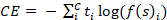
Identifying an object among many other categories is becoming a popular application that can be used to expose new information in image data. By using ZSL, a target class is recognized and interpreted even when a similar object has not been seen or there is no information regarding the category it belongs to. ZSL methods are made to study various object classes, their features, and use the features learnt during image classification to help recognize unseen classes of data. It uses information from the training classes with labelled samples using the class attributes to perform recognition tasks. It is performed in the following way: • training stage: the stage where information regarding the data is extracted, • learning stage: the stage where the information captured categorizes various data samples which have not been previously seen. The ZSL process is quite similar to how humans recognize objects. But there can be projects where data of thousands of classes may need to be labelled manually. Using the process of ZSL, it is feasible to classify many objects instead of performing recognition tasks on finite sets of objects. Traditional object classification tasks may struggle to provide good results when there is a lack of relevant data. In these types of situations, ZSL can potentially be used to implement many innovative applications. While implementing ZSL, let us assume that we are training the model for C classes. The activation function used is the Softmax function. Since we are using it for a multi-class classification, the output will be the probabilities of every class, with the target class having the highest probability. We minimize the objective functions using Categorical Cross-Entropy Loss9. It is a good metric for differentiating between two discrete probability functions. Categorical Cross-Entropy Loss is defined as:
which is the Softmax function. where s represents the input vector, esi is the standard exponential function for input vector, C is the number of classes in the multi-class classifier and esj is the standard exponential function for output vector. The Categorical Cross-Entropy Loss: where f(s)i is the i-th scalar value in the model output, ti is the corresponding target value and C is the number of scalar values in the model output. The vector of the target class is compared with the vectors of training classes to obtain the predictions at the testing phase.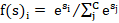
DESIGN OF THE PROBLEM
Consider a scenario where it is wished to classify species which live in places that humans cannot go to easily. It is almost impossible to collect the necessary image data of these animals. It would not be enough if you just collected similar pictures because it would not provide the diversity that the recognition task needs. So, the image data has to be quite unique. Adding to this difficult task of classifying various target categories, labelling of target categories can be trickier than it may seem. There are cases in which the labelling of object classes can only be done after the topic is really mastered or in the presence of a specialist. Under the guidance of a person who is experienced in the particular field, object classification tasks like the classification of endangered animals or plants are viewed as examples of giving labels to the data. Let us consider pandas, where some specific species of pandas are considered to be endangered or vulnerable, but an ordinary human will label all the pandas they observe as a panda instead of correctly naming its exact species which can only be done by an expert. Although there is truth in labelling it as just a panda, it does not help the neural network to recognize a particular species of panda. In such a situation, all the generalized labels are pretty much useless and there is the need of a specialist to label the particular species. As labelling the data instances manually can take a lot of time, ZSL can be used to perform classification tasks in such scenarios. To perform object classification tasks with good accuracy in fine-grained object classification, it is needed to decide on a finite amount of target categories. It is important to gather as much image data for the target categories that have been decided. The training dataset must obviously have images captured at various positions in diverse habitats. Even though image data of a lot of object classes can be collected, there are often classes in which data is difficult to get hold of.
METHODOLOGY
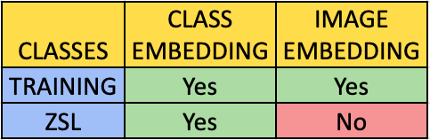
While performing ZSL on image samples that have not been trained on may seem strange at first, it is possible to do so. The Training and Zero-shot classes are then separated. Simply put, how is it possible to recognize objects that the model has not seen before? The data should be depicted with sensible features. Thus, two data depictions are used. Class embedding and image embedding are the two data depictions that are required. Image embedding10 is used to read images and evaluate them locally or to upload them to a remote server. To calculate a feature vector for each image, deep learning models are used. This is done so in order to return another data table with additional image descriptors. This is learnt using a deep learning model and is called a feature vector. The deep learning model can either be a pre-trained convolutional network that already has a high accuracy rate or a new one can be built from scratch. For the image feature extraction process, a pre-trained deep learning model called VGG162 is used. Image embeddings can be obtained for all the instances of the dataset that are collected for training classes. But there is a lack of samples of images for the ZSL classes. It is impossible to obtain image embeddings for the ZSL classes. It is here where ZSL is different from the usual image classification problems. Now in this stage, there has to be an alternative depiction of data linking both the ZSL and training classes. Image embedding should be learnt from the image dataset regardless of which class they belong to, whether it be training or Zero-shot. Therefore, labels of categories should be focused upon instead of concentrating on the image itself. Both the class labels and image samples for the Training classes are available to us now. However, only the class labels for the Zero-shot classes are available as the image data has not been seen. This is shown in Figures 1 and 2. Here, it can be seen that image embedding is done only for the training classes and not for the ZSL classes, while class embedding is done for both training and ZSL classes.
MODEL ARCHITECTURE
As the final step is using the Word2Vec as a link to classify the target categories that have not been trained on, the last layer of the model that was custom-defined and untrainable is removed. The model then gives a vector output for each input image. The model contains various layers, and it is made sure that the input shape of the first layer of the model is of the same shape as the image attributes extracted using the VGG16 model. A vector is then obtained that gives an indication of a coordinate in the Word2Vec space for every data instance. Then this vector output is mapped to the one which is placed closest by differentiating it with the thirteen category vectors available. From the VGG16 model, the last three layers were removed in order to map to the input shape of the custom sequential model which is as shown in Figure 3. After tuning the hyperparameters11 and getting to the best possible model performance, the trained model is tested on the image data of ZSL classes.
DATA COLLECTION
The first step is to collect the necessary images of both the training and testing classes. The image data of training classes is utilized for training the ZSL model, while that of the testing classes is utilized for assessing how the model performs.
The image data described above is collected from Google Images and Kaggle23. Thirteen classes were selected in total, out of which nine classes are chosen for the training phase and four classes are chosen as ZSL classes. Now, it is necessary to decide which classes out of the total thirteen are chosen to be ZSL and training classes. Various food dishes have been picked as classes for demonstrating the process of ZSL for classification of unseen objects.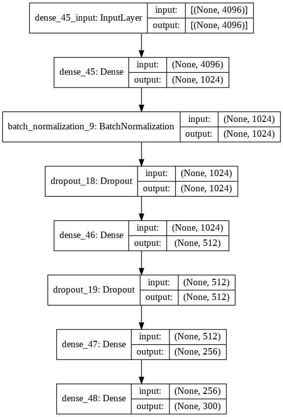
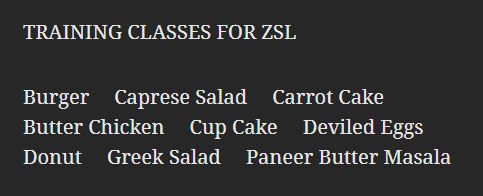
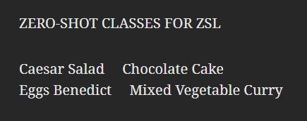
IMAGE FEATURE EXTRACTION
From Google Images and Kaggle, the required food dish images are obtained for all the necessary classes. Extraction of the image attributes1 is done using the VGG16 convolutional neural network2 from the data collected.
WORD EMBEDDINGS
The word embeddings12 of all the classes are gathered after the datasets have been formed and extracted the image features. Google’s Word2Vec depiction is used for this process. This is a Word2Vec for all the 13 food dish target categories which have been considered. Class embedding is the form of depiction of a particular category in a vectorized manner. It can be easily accessed for every object category aside from image embeddings. Vectors are placed near each other in the Word2Vec space if the two words tend to appear together in similar Google News documents.
From the Word2Vec space illustrated in Figure 6, it can be noticed that the vectors of food dishes related to cakes are placed near to each other. But they are placed far from the vectors of food dishes related with salads.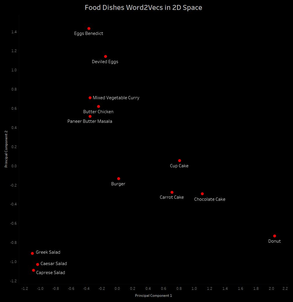
MODEL TRAINING
Here, the inputs are the image features extracted, and the corresponding outputs are the Word2Vecs. A fully-connected Keras model is created as a follow-up to the pre-trained convolutional model, which is used to extract the image features. The last layer of the model created has to be a custom layer. This layer should not be trainable. This indicates that the layer must not be changed by updating the gradients. The different kinds of layers used in this model are: • dense layer: It is a deeply connected neural network layer. It is the most frequently used layer in deep neural networks. It receives input from all neurons of its previous layer13, • dropout layer: It is a method of reducing overfitting in neural networks by preventing the model from learning noise in the dataset14, • batch Normalization layer: It is a method that is used for training neural networks which standardize the inputs to a layer for each mini-batch15. The formula for implementing Batch Normalization is:
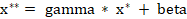
where x* is the new value of a single component, E[x] is its mean and var(x) is its variance. Batch Normalization can learn the identity function using: where x** is the final normalized value.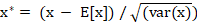
OPTIMIZERS
The process of updating the deep learning model according to the loss function’s output by tying together the parameters and the loss function is performed by optimizers. Simply put, by futzing with the weights of the neurons, the deep learning model is updated to its best form. The model is trained using various optimizers in order to know which best fits the dataset. The accuracies obtained are shown in Table 1.
| Optimizer | Top-5 Accuracy | Top-3 Accuracy |
| Adagrad | 0,92 | 0,78 |
| Adam | 0,91 | 0,76 |
| SGD | 0,90 | 0,76 |
| Nadam | 0,89 | 0,76 |
| RMSprop | 0,88 | 0,75 |
Here, it can be observed that the Adagrad optimizer16 performs best on our training dataset with the best Top-5 and Top-3 accuracy. The Adam optimizer17 comes a close second after Adagrad. Adagrad (Adaptive Gradient Algorithm) is an algorithm that is used for gradient-based optimization. By incorporating knowledge of past observations, the learning rate is adapted to the parameters component-wise. It performs bigger updates for those parameters which are not frequent and smaller updates for those that are frequent. While using Adagrad, the learning rate need not be tuned manually, and its convergence is more reliable. Adagrad is also not sensitive to the size of the master step. The formula used by Adagrad to update the parameters is13:
where t is the time step, ϴ is the weight/parameter which we want to update, vt denotes different learning rates for each weight at each iteration, α is a constant number and ∂L/∂ϴt is the gradient of L, the loss function to minimise, with respect to ϴ.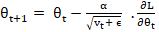
RESULTS AND ANALYSIS
The accuracy scores of the deep learning model when it is tested on the image data of the four unseen food dish classes are shown in Figure 7. 92% accuracy for Top-5 predictions and 78% for Top-3 is attained after tuning the hyper parameters of the deep learning model.
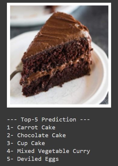
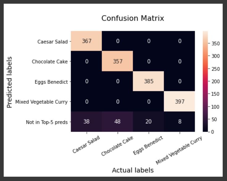
For testing the model, the data instances of ZSL classes will be used. These images have not been used for training the model. The deep learning model is evaluated by performing ZSL classification on the collected image data. The Word2Vec is compared for each image sample with the 13 vectors. The metric that is used is Euclidean distance10. Finally, the class which is closest to the target class in the Word2Vec space is predicted. For example, an image of a Chocolate Cake is taken which is one of the zero-shot classes. The predictions of the model are shown in Figure 8 upon performing ZSL on the selected image. It can be seen that it predicts ‘Chocolate Cake’ at the second position while not having seen the image class during the training process. The metric that is being used to evaluate the model is Top-5 and Top-3 accuracy. It basically means whether the actual label for the unseen image is present in the Top-5 or -3 predictions. Top-5 accuracy is around 92 %. Since this is a process of classifying images that have not been seen by the model before, the accuracy percentages are prety decent. The deep learning model knows only the positions of the classes in the Word2Vec space. Thus, it can be deduced that ZSL clearly works better than some random object recognition task. A confusion matrix helps in visualizing the performance of a deep learning model. Figure 9 shows how many images the model predicted correctly for each class. The ‘Not in Top-5 preds’ row indicates the number of images the model predicted incorrectly for each class.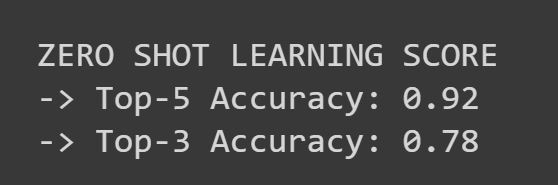
EFFECT OF BATCH SIZE
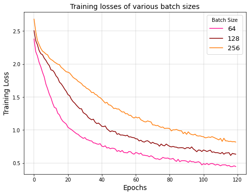
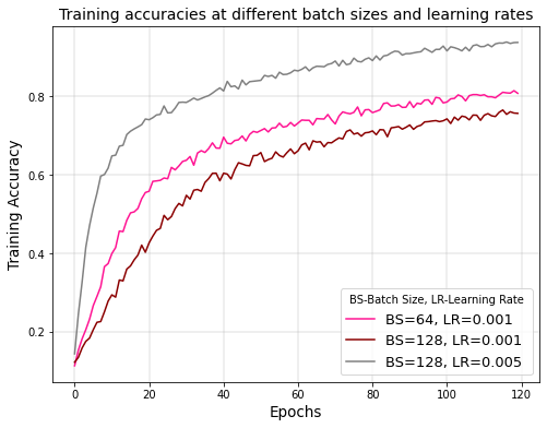
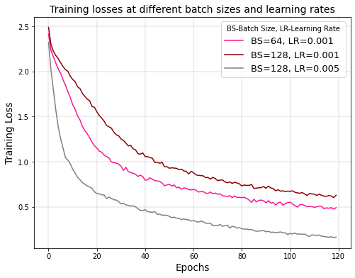
The amount of data instances that are needed to be trained before updating the necessary hyperparameters is known as batch size. It iterates over the data and predicts classes. The predicted values are compared to the expected values and the loss is computed. The neural network is improved from this loss by moving down the error gradient. The training accuracies and losses of different batch sizes such as 64, 128 and 25618 are compared. The training accuracy and loss of the deep learning model using various batch sizes are shown in Figures 10 and 11. The number of epochs (X-axis) denote the number of passes that the model has completed of the entire training dataset.
From the figure one can analyse that low training accuracy is caused by high batch sizes. As the batch size increases, the training accuracy decreases and the training loss increases. This is due to the amount of data being trained as a batch is increased. A hypothesis on why this happens is that the training instances of a particular batch interfere with one another’s gradient. Therefore, this leads to smaller gradients overall.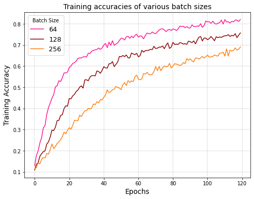
EFFECT OF LEARNING RATE
The hyperparameter that controls the amount of change in reaction to the loss every time the weights of neurons get updated is called the learning rate11. The process of selecting a learning rate can be difficult as the value may be too large, resulting in learning a sub-optimal set of weights too quickly, whereas a smaller value may end in the training process getting stuck. There are studies19 that analyze the impact of varying learning rates over larger batch sizes. Thus, the learning rate is increased and it is checked if the training accuracy that has been lost are regained.
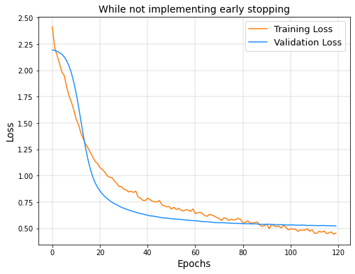
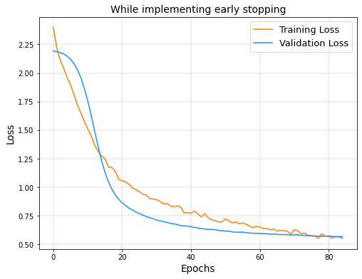
IMPLEMENTING EARLY STOPPING
The process of monitoring the model’s performance for each epoch on a validation set during training and ending the training based on the validation set performance is called Early Stopping20. Early Stopping is implemented during training and it is checked whether there is an improvement in the Validation loss. In Figure 14, it can be seen that the validation loss stops decreasing and starts to go back up. This shows that the model is overfitting the dataset. However, in Figure 15 implementing Early Stopping, the training is stopped as soon as the validation loss starts to increase, thereby preventing overfitting.
To help the model in generalizing well, regularization layers are used that make some changes to the algorithm. Here, in the methodology for optimization, the following regularization layers are implemented: Dropout, Gaussian Noise and Gaussian Dropout. Dropout14 is partially learning the weights over many epochs. Dropout value of 0.5 leads to the highest possible regularization. The intention is to lessen the dropout loss in order to regularize the deep learning model. This is done using the following equation:


| Regularization layer | Top-5 Accuracy | Top-3 Accuracy |
| Dropout | 0,92 | 0,78 |
| Gaussian Noise | 0,91 | 0,76 |
| Gaussian Dropout | 0,88 | 0,72 |
As it can be observed that using the Dropout layer achieves the best results, with the Gaussian Noise layer coming a close second. Two Dropout layers are used with the first one having a rate of 0,8 and the second one having a rate of 0,5. The rate of the first layer is 0,8 because it is important to retain as much information when implementing Dropout layers at the input. If not done so, a lot of information might be lost and it might affect the training process.
CONCLUSIONS
A ZSL model is built in a way that uses the VGG16 model2 to extract image attributes and then recognize daily life objects which the model has not seen. Nine training classes and four ZSL classes were considered in this article to classify the samples of ZSL classes on training the model with samples of training classes. The data is collected from scraping Google for images and from a Kaggle dataset. A deep learning model is then trained on the features extracted from the training class data collected. It is tested on ZSL class data and achieved a Top-5 accuracy of 92 %. Images that have not been trained on are being classified, especially when the neural network is not aware of the ZSL classes, at scores that are quite decent. The only information given to the model is location of the word vectors of these classes in the Word2Vecs. The scores are not always high as it is more difficult to recognize target classes that belong to similar categories. ZSL has great scope and is a popular topic in Deep Learning even though it is a relatively new idea. ZSL can be built upon and improved to make further systems like helper-based systems using ZSL for the visually impaired. The natural vegetation can be analysed in remote areas and rare animals can be classified in their own habitats. There have been a lot of developments recently in the field of robotics22 and ZSL can be used to produce robots that can carry out functions of humans. This can be done as humans can recognize an object that the model has not been trained on before and might not have information regarding what the thing is. Future work that we envisage carrying out is focused on adopting ZSL mechanisms in deep learning algorithms for the design and development of intelligent systems. We aim to test other N-shot approaches such as one-shot and few-shot learning, and compare their performance to ZSL. Another approach could be to combine other N-shot approaches with ZSL to achieve better predictions in practical situations such as autonomous vehicles. This takes the novelties of all such approaches and produces an overall positive result. The code is available athttp://www.github.com/JatinArutla/Zero-Shot-Learning.