
1. Introduction
The intensive development of urban centres, industry, agriculture, as well as the rise in living standards of the people, is necessarily accompanied by increasing quantities of solids, liquid and gaseous waste materials in water. In order to mitigate the potential effects of the hazard on human health, constant monitoring of water quality is legally required. Particular attention should be paid to the water that are used daily by anyone for household purposes or as some form of recreation. The varied nature of the hazards to human health and well-being posed by recreational waters demands a full audit of the relative importance of the resultant health effects and the resources (Chen et al., 2020; Updyke et al., 2015). Surface and coastal waters are used for a variety of leisure and recreational activities and for many other purposes like transportation medium, food production, hydroelectricity generation, as well as a repository for sewage and industrial waste. Such activities are not always compatible with one another. Water and its recreational uses have significant and major influences on human health and well-being. Water pollution has been very widespread under which it implies a decrease in water quality due to subsequently received specimens. Pollution in a sense implies the degradation of quality water by physical, chemical, biological or radiological contamination to the extent that it is impossible its use and such water is harmful to human health. Biological contamination of water includes the presence of pathogenic bacteria such as Escherichia ( E. coli) and intestinal enterococci, which, in water, come from faecal waters and can cause some intestinal diseases (Rossi et all., 2020; Uprety et all., 2020). Total and fecal coliforms , E. coli and enterococci are fecal indicator bacteria (FIB) that are typically used to assess water quality. Epidemiology studies show that the exposure to recreational waters contaminated with FIB from wastewater and urban runoff correlates with risk of diarrheal illness, respiratory disease, and skin ailments (Arnold et al., 2016; Colford et al., 2007; Korajkić et al., 2018; Wanjugi et al., 2016). The pathogenic micro-organisms that can be found in water bodies have a wide range of sources. These include sewage pollution, organisms naturally found in the water environment, agriculture and animal husbandry and the recreational users themselves. Sewage of domestic origin comprises a particularly unhealthy mixture of microorganisms. The microbiological hazards encountered in water-based recreation include viral, bacterial and protozoan pathogens. Primary concern has usually been directed towards gastro-intestinal illnesses acquired from recreational waters, although acute febrile respiratory illness and infections of eyes, ears, nose and throat have all been identified as acquired through bathing. In terms of international standards, the World Health Organization (WHO) published the “Guidelines for Safe Recreational Water Environments” with an Addendum in 2009 (Word Health Organization, 2009). The guidelines recommended jurisdictions to conduct microbiological water quality assessment (MWQA) and sanitary inspections to classify the likelihood for human sewage versus other fecal sources in bathing waters. Another major international guideline for recreational water classification is the European Union (EU)’s Directive 2006/7/EC (Official Journal of the European Union, 2006), which classifies coastal waters into “Excellent quality”, “Good quality”, “Sufficient” or “Poor”, with reference to the abundance of both intestinal enterococci and E. coli measured over four bathing seasons (Table 1).
Table 1. Classification criteria for coastal and transitional waters under the EU’s scheme
In order to determine the number of microorganisms in bathing water at two lakes in Zagreb (Bundek and Jarun), a sample of water is taken at nineteen locations over three years, of which three were taken at Lake Bundek and sixteen at Lake Jarun. The aim of this study was to examine the correlation between microbiological indicators of water quality E. coli and intestinal enterococci with the sampling location using statistical mathematical models.
2.1. Study sites and sampling collection
The lakes (Bundek and Jarun) were created by gravel exploitation and after the ending of exploitation, the lakes became a bathing area, Figure 1.

Figure 1. Bundek and Jarun lakes
For testing the water quality of Bundek Lake, samples were taken in the Big Lake region (marked as A), Figure 2. Three sampling points were selected, the eastern shore of the lake (B1), the western shore of the lake (B2) and the southern shore of the lake (B3).
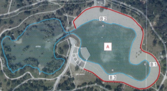
Figure 2. Sampling location at Bundek Lake
Table 2 shows that in 2014 the samples were taken twice before the bathing season, one day before the official start of the season (10.06.), four times during the season and once at the very end of the season (08.09.). In 2015 and 2016, pre-bathing sampling was performed only once, while the rest of the sampling was conducted as in 2014.
Table 2. Sampling dates at Bundek lake and Jarun lake from 2014 to 2016
| 2014. | 2015. | 2016. |
|---|---|---|
| 2.4. | 14.4. | 12.4. |
| 21.5. | 9.6. | 9.6. |
| 10.6. | 23.6. | 24.6. |
| 30.6. | 7.7. | 7.7. |
| 7.7. | 21.7. | 19.7. |
| 21.7. | 3.8. | 9.8. |
| 11.8. | 24.8. | 23.8. |
| 26.8. | 7.9. | 9.9. (Only Jarun lake) |
| 8.9. |
For determination of the water quality at Jarun Lake (Figure 3.), samples were taken in the area of Big and Small Lakes. Six sampling points (TU01 - TU06) were selected for sampling in the Big Lake area, six samples were also taken at Small Lake (TU07 - TU12), two samples (TU13 and TU14) were taken on the Rowing Island and Trešnjevka Island, and two samples (TU15 and TU16) were taken on the Universiade Island.

Figure 3. Sampling location at Jarun Lake
In the area of Jarun Lake, samples, with a total of sixteen sampling points, were taken nine times in 2014, while in 2015 and 2016, samples were taken eight times. Table 2. shows the exact sampling dates.
It can be seen from Table 2. that the samples in 2014 were taken twice before the bathing season, one day before the official start of the season (10.06.), four times during the season and once at the very end of the season (08.09.). In 2015, pre-bathing sampling was performed only once, while the rest of the sampling was performed as in 2014. The same was the case in 2016, one sampling was done before the season, while the other seven were sampled the same as in previous years. A total of 500 mL of water sample was collected at each defined sampling point at a water depth of 0.5 m below the water surface within the designated bathing area for each lake. The sampling equipment were sterilized and sample bottles were also sterilized in an autoclave at 121 °C for 15 min. Water samples were kept at a temperature of around 4 °C in a cooler box and sent to the laboratory for testing according to the standard norm (Official Journal of the European Union, 2006; ISO 19456:2006; ISO 9308-3:1998)).
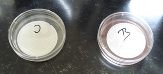
Figure 4. Membrane filters on CC agar and Slanetz-Bartley agar before incubation
These are selective nutrient media, which means that they are specific to that bacterial species only. In addition to E. coli (blue colonies), total coliforms (pink colonies) also grow on CC agar. Nutrient media were incubated at 37 °C and bacterial colonies growth was identified after 24 hours (the first reading), while the second reading was performed after 48 hours (confirmatory test). The confirmatory test for E. coli is a biochemical series (Figure 5.) that is designed to confirm the presence of E. coli due to the possible growth of similar colonies. E. coli is planted on five different nutrient media with CC agar.
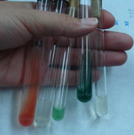
Figure 5. Nutrient media for the biochemical array (left to right: double sugar, SIM, urea, citrate, Clark)
The confirmatory test for intestinal enterococci is performed by taking a membrane filter with colon membrane filter, which is transferred with sterile forceps to a heated plate with bile esculin agar. The plates were incubated at 44 °C for 2 hours. The test is positive if black spots are observed that occur due to esculin hydrolysis. The bacterial colonies are then counted.
3. Methods
Analysis of variance (ANOVA) is a statistical procedure that allows one or more factors to be examined simultaneously in a large number of groups of subjects. In other words, ANOVA is a criterion that shows whether differences between groups are accidentally greater than differences within groups. The analysis of variance was first developed by the famous English statistician R. A. Fisher. Today, ANOVA is a very important and popular method for investigating various random phenomena in many scientific fields (Mahmoud et al., 2014; Johnson and Wichern, 2007; Hoffman, 2019). The very name „analysis of variance” comes from the fact that it compares the variance between different groups with the variability within each group. It is most commonly used to determine whether there are differences between several arithmetic means and whether these differences are statistically significant or random. According to the number of factors that affect the resulting trait, analysis of variance can be one-factor (one-way), two-factor (two-way) and multifactorial.
In this paper we shall deal with one-way ANOVA. At first, we have assured that the following assumptions for using ANOVA are valid: random variables must be independent, the distribution of the basic set has to be normal with equal variance. For comparison, we have made also two non-parametric statistical tests: Kruskal-Wallis and extended median test. Kruskal-Wallis test is a non-parametric test used when random variables are not normally distributed, and by means of ranks, it is necessary to examine whether the basic sets have equal medians.
Extended median test investigates if three or more basic sets have equal median (Johnson and Wichern, 2007).
4.1. Processing and exposure of microbiological indicators by sampling points
Two microbiological indicators, E. coli and intestinal enterococci, were determined in water samples. Based on the results of microbiological indicators, logarithmic values of E. coli and intestinal enterococci ratio were calculated for better transparency.
Below are box and whisker plots for both microbiological parameters from 2014 to 2016 (Figure 6-8) divided into three groups. There are sampling points on the abscissa axis, and on the ordinate axis is the logarithmic value of the microbiological indicator.
The microbiological indicators ratios are shown in the box and whisker diagram because of the large amount of data. At Lake Bundek, 25 samples were taken for each sampling point (B1, B2, B3) over the three years, so there is a total of 75 samples. Figure 6a) shows that the distribution of E. coli for location point B1 ranges from 1.3 to 3 and the distribution is symmetric. 25 % of E. coli observations are less than 1.7, while 25 % are greater than 2.5. On average, the amount of E. coli at location B1 is 2.123. Since there is no value below the lower and upper edges of the mustache, it can be concluded that there are no outliers (Heikka, 2008; Fange et al., 2017). Distribution for location point B2 ranges from 1.3 to 2.8, with distribution skewed to the right. 25 % of observations are less than 1.6 and 25 % are greater than 2.2. On average, the amount of E. coli at location B2 is 1.901. Below the lower edge of the mustache there is one observation, which is designated as an outlier (the value for E. coli is 1.3). Distribution at location point B3 ranges from 1.05 to 3.0. The distribution is slightly skewed to the right. 25 % of observations are less than 1.6 and 25 % are greater than 2.65. The average value of E. coli in location point B3 is 2.073. Since there is no value below the lower and upper edges of the mustache, it can be concluded that there are no outliers. The range of variation within 50 % of the distribution is the largest at location B3 and the smallest at location B2.
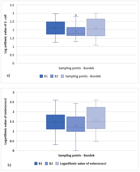
Figure 6. a) Box and whisker plot for E. coli at Lake Bundek
Figure 6b) shows the distribution of enterococci amount at location B1 to B3. It ranges from 0 .3 to 2 .6 and is symmetric. On average, enterococci at B1 are 1 .474 . 25 % of observations or enterococci counts are less than 1 .1 and 25 % are greater than 1 .8 . Below the lower edge of the mustache, there are two observations, that is, two outliers (enterococci: 0.48 and 0.3). The distribution for point B2 ranges from 0 to 2 .4, skewed to the right. 25 % of observations are less than 1 and 25 % are greater than 1 .75 . The enterococci amount averages 1 .291 . Below the lower edge of the mustache, there are three observations that are labeled as outliers. The distribution range at location B2 is from 0.49 to 2.6 and is slightly skewed to the right. The average of enterococci for B2 is 1.570. 25 % of observations are less than 1.15 and 25 % are greater than 2.25. Below the lower edge of the mustache is a single projectile (enterococci 0.48). The range of variation within the mean 50 % of the distribution is the largest for location B3 and the smallest for location B1.
At the Great Lake (Jarun), 25 samples were taken at six sampling points (TU01, TU02, TU03, TU04, TU05, TU06), i.e. 150 samples in total (Fig. 7). The amount of E. coli and enterococci is shown in Figure 7a) by a box and whisker diagram. It ranges from 1.15 to 2.45 and is slightly beveled. 25 % of observations are less than 1.6 and 25 % are greater than 2.45. On average, the amount of E. coli at location TU01 is 2,017 and there are no outliers. Distribution for location TU02 ranges from 1.15 to 2.8 and is slightly skewed to the left. 25 % of observations are less than 1.3 and 25 % are greater than 1.95. The amount of E. coli at TU02 averages 1.705. Since there is no value below the lower and upper edges of the mustache, it can be concluded that the outliers do not exist. The distribution shown in Figure 7a) for location TU03 ranges from 1.15 to 2.55 and is slightly skewed to the right. 25 % of observations are less than 1.49, while the other 25 % is greater than 2.2. The average value of E. coli is 1.809. Distribution for location TU04 (Great Lake, Jarun) ranges from 1.15 to 2.55 and is slightly skewed to the right. On average, the amount of E. coli at TU04 is 1,676. 25 % of observations are less than 1.49 and 25 % are greater than 2.2. Below the lower edge of the mustache are five observations, four with 1.18 and one with 1.19. For location TU05 the distribution ranges from 1.15 to 3 and is very skewed to the right. 25 % of observations are less than 1.2 and 25 % are greater than 2.05. The average amount of E. coli is 1.688; The distribution for location TU06 on the Great Lake Jarun ranges from 0.7 to 3, with the distribution slightly skewed to the right. 25% of observations are less than 1.45 and 25 % are greater than 2.5. On average, the amount of E. coli at TU06 is 1.934. Below the lower edge of the mustache there is one observation, which is designated as an outlier ( E. coli 0.7) The range of variation within the mean 50 % of the distribution is the largest for location TU06 and the smallest for location TU04.
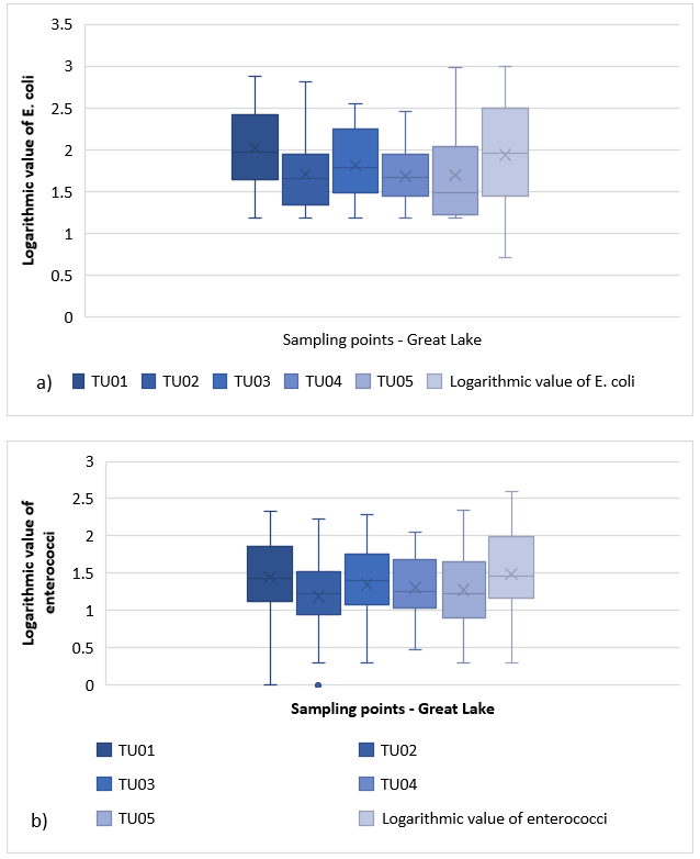
Figure 7. a) Box and whisker plot for E. coli at Great Lake (Jarun)
The distribution of enterococci at Great Lake (Figure 7b)) ranges from 0 to 2.3, slightly skewed to the right. 25 % of enterococci value is less than 1.1, while 25 % is greater than 1.9. The average enterococcus value at TU01 is 1,442. Below the lower edge of the mustache, there are two observations (enterococci 0 and 0.3). The distribution for location TU02 on the Great Lake, Jarun ranges from 0.3 to 2.2, the distribution slightly skewed to the left. 25 % of observations are less than 0.95 and 25 % are greater than 1.5. The average enterococcus value at TU02 is 1.185. Below the lower edge of the mustache, there are four observations that are labeled as outliers (two enterococci 0.3 and 0 and 0.6, respectively). At the location of TU03, the enterococci distribution ranges from 0.3 - 2.3, with the distribution slightly skewed to the right. 25 % of observations are less than 1.1 and 25 % are greater than 1.8. The enterococci average is 1.352. At the TU03 site below the lower edge of the mustache, there are three observations (enterococci 0.3 and 0.48 and 0.6, respectively). The enterococci range for location TU04 ranges from 0.5 to 2.05 (skewed to the right). The average amount of enterococci at this location is 1.308. 25 % of observations are less than 1.05 and 25 % are greater than 1.7. Below the lower edge of the mustache are three observations that are labeled as outliers (enterococci amount 0.48, 0.6, and 0.7). The distribution for location TU05 on the Great Jarun Lake ranges from 0.3 to 2.35, with the distribution slightly skewed to the right. 25 % of observations are less than 0.9 and 25 % are greater than 1.7. On average, enterococci at TU05 are 1.274. Below the lower edge of the mustache there is one observation, which is referred to as an outlier (enterococcus 0.3). The range of enterococci at TU06 ranges from 0.3 to 2.6. On average, enterococci at TU06 are 1,491. 25 % of observations are less than 1.2 and 25 % are greater than 2. Below the lower edge of the mustache are three observations that are labeled as outliers (two enterococci with 0.3 and 0.7). The variation range within the mean 50 % of the distribution is the largest for location TU06 and the smallest for location TU02.
At Small Jezero (Jarun), 25 samples were taken at six sampling location (TU07, TU08, TU09, TU10, TU11, TU12) and the amount of E. coli and enterococci is shown in Figure 8 by a box and whisker diagram. The distribution of E. coli ranges from 1.1 to 2.85 and is heavily skewed to the right (Figure 8a)). 25 % of E. coli is less than 1.2, while 25 % is greater than 2.4. The average amount of E. coli is 1,738. To location TU08, the distribution is in the range 1.2 - 2.8, and is heavily skewed to the right. 25 % of observations are less than 1.49 and 25 % are greater than 2.25. The E. coli average on TU08 is 1.870. The outliers do not exist. Distribution at TU09 ranges from 1.18 to 3.0. The distribution is slightly skewed to the left. The average E. coli value at this location is 1.928. 25 % of observations are less than 1.2 and 25 % are greater than 2.5. Since there is no value below the lower and upper edges of the mustache, it is concluded that there are no outliers. The distribution for the TU10 site in Small Lake, Jarun ranges from 1.2 to 3, with the distribution slightly skewed to the right. 25 % of observations are less than 1.7 and 25 % are greater than 2.4. On average, the amount of E. coli at TU10 is 1,989. Below the lower edge of the mustache, there are four observations that are designated as outliers (four quantities of E. coli 1.18). The distribution for point TU11 ranges from 1.2 to 2.9. The distribution is slightly skewed to the right. The average E. coli value for TU11 is 1.919. 25 % of observations are less than 1.5 and 25 % are greater than 2.4. At TU12, the distribution ranges from 1.2 to 2.9 and is slightly skewed to the right. 25% of observations are less than 1.9 and 25 % are greater than 2.5. The average value of E. coli is 2.163. Below the lower edge of the mustache are two observations of the so-called outliers (quantity of E. coli = 1.18). The range of variation within the mean 50 % of the distribution is the largest for location TU09 and the smallest for location TU12.
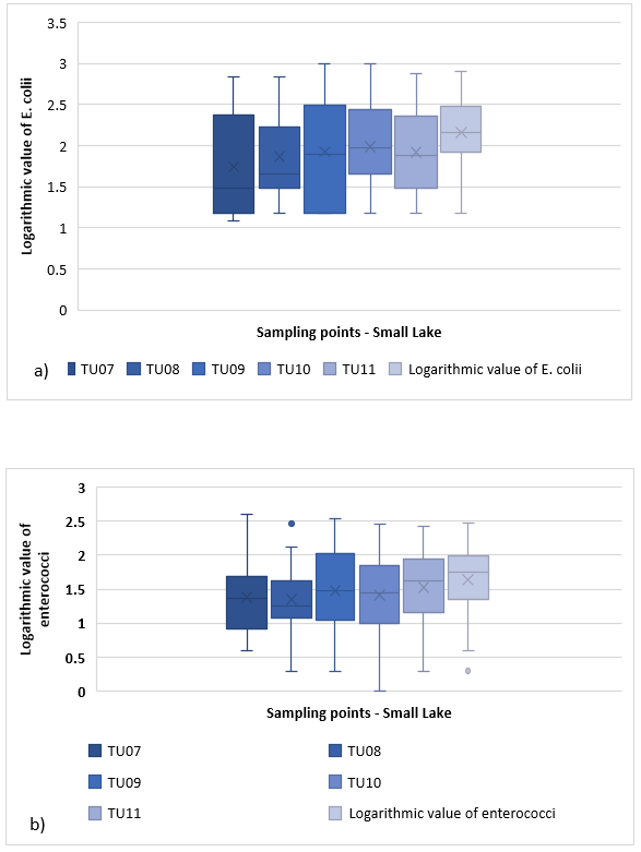
Figure 8. a) Box and whisker plot fo E. coli at Small Lake (Jarun)
The enterococci quantity (Figure 8b)) at location TU07 ranged from 0.6 to 2.6, the distribution skewed to the left. The average enterococcus value at TU07 is 1.386. 25 % of observations are less than 0.9 and 25% are greater than 1.7. There are no outliers at this location. The distribution for the TU08 site at Small Lake, Jarun ranges from 0.3 to 2.1, the distribution skewed to the right. 25 % of observations are less than 1.1 and 25 % are greater than 1.6. On average, enterococci at TU08 are 1.347. Below the lower edge of the mustache, there are two observations that are marked as outliers (enterococci are 0.3 and 0.48), above the upper edge of the mustache is one observation (enterococci is 2.46). The enterococcus value at location TU09 ranges between 0.3 and 2.55. The distribution is slightly skewed to the right. The percentage of 25 % of observations is less than 1.05, while the other 25 % is greater than 2. The average value of enterococci is 1.480. Below the lower edge of the mustache there is one observation marked as an outlier (enterococcus 0.3). At TU10, the enterococcus range ranges from 0 to 2.49, with the distribution slightly skewed to the left. 25 % of observations are less than 1 and 25 % are greater than 1.9. On average, enterococci at TU10 are 1.411. Below the lower edge of the mustache is one observation, which is referred to as outlier (enterococci is 0). The range of enterococci at TU11 is between 0.3 and 2.4. The average value of enterococci is 1.528. 25 % of observations are less than 1.1 and 25 % are greater than 1.9. At the TU11 site, there is one observation marked as an outlier (enterococcal amount: 0.3). Location marked as TU12 distributes in the range 0.6 to 2.45. The distribution is skewed to the left. There are three observations below the lower edge of the mustache (enterococci 0.3, 0.6, and 0.85). 25 % of observations are less than 1.35 and 25 % are greater than 2. The average enterococci value is 1.641. The variation range within the mean 50 % of the distribution is the largest for location TU09 and the smallest for location TU08.
Analysis of variance of the microbiological parameters at the sampling points
When calculating the one-factor analysis of variance in all samples, the level of significance α = 0 .05 was used. The level of significance can be defined as the probability of a decision to reject the null hypothesis when the null hypothesis is actually true.
Before calculating the one-factor analysis of variance for E. coli, it is assumed that all arithmetic mean values at all three examined locations (B1, B2, B3) are equal:
H0: µ (B1, E. coli) = µ (B2, E. coli) = µ (B3, E. coli)
An alternative hypothesis is:
H1: at least one of µ (B1, E. coli), µ (B2, E. coli), µ (B3, E. coli) is different than others.
The p-value (Table 3) calculated by ANOVA is p = 0 .256 > α, which means that there is no statistically significant difference between the dependent variable mean values regarding to the three examined locations. Although there is a difference between groups, there is no statistically significant difference in the deviation of the level of E. coli presence with respect to the sampling points. The table shows that the critical value of test statistics (3.124) is greater than the value of test statistics (1.389) and according to the rules for one-factor analysis of variance the assumption is accepted, i.e., arithmetic values obtained from samples do not depend on the sampling location.
Table 3. Dependence of the arithmetic mean of E. coli on the sampling points at Lake Bundek
A one-factor analysis of variance was performed to investigate the existence of a difference in the level of presence of intestinal enterococci with respect to sampling points.
H0: µ (B1 , enterococci ) = µ (B2 , enterococci ) = µ (B3, enterococci )
An alternative hypothesis is:
H1: at least one of µ (B1 , enterococci ), µ (B2 , enterococci ), µ (B3, enterococci ) is different than others.
The p-value (Table 4) calculated by ANOVA is p = 0 .250 > α, which means that there is no statistically significant difference between the dependent variable mean values regarding to the three examined locations. The table shows that the critical value of test statistics (3.124) is greater than the value of test statistics (1.415) and according to the rules for one-factor analysis of variance the assumption is accepted, i.e. arithmetic values obtained from samples do not depend on the sampling location.
Table 4. Dependence of the arithmetic mean of enterococci on the sampling points at Lake Bundek
| Scattering source | df | Sum of squares | Variance estimate | F-value | p-value | Critical value |
|---|---|---|---|---|---|---|
| Between groups | 2 | 1.008 | 0.504 | 1.415 | 0.250 | 3.124 |
| Within groups | 72 | 25.639 | 0.356 | |||
| Total | 74 | 26.647 |
The hypothesis for the arithmetic value of E. coli at Great Lake Jarun are:
H0µ (TU 01 , E. coli) = µ (TU 02 , E. coli) = µ (TU 03 , E. coli) = µ (TU 04 , E. coli) = µ (TU 05 , E. coli) = µ (TU 06 , E. coli)
An alternative hypothesis is:
H1: at least one of µ (TU 01 , E. coli), µ (TU 02 , E. coli), µ (TU 03 , E. coli), µ (TU 04 , E. coli), µ (TU 05 , E. coli), µ (TU 06 , E. coli) is different than others.
The p value is greater than the value of α, 0 .062 > 0 .05 . The critical value of test statistics (2.277) is greater than the value of test statistics (2.160), and according to the rules for one - factor analysis of variance, the H0 hypothesis is accepted.
Table 5. Dependence of the arithmetic mean of E. coli on the sampling points at Great Lake Jarun
| Scattering source | df | Sum of squares | Variance estimate | F-value | p-value | Critical value |
|---|---|---|---|---|---|---|
| Between groups | 5 | 2.549 | 0.510 | 2.160 | 0.062 | 2.227 |
| Within groups | 144 | 33.993 | 0.236 | |||
| Total | 149 | 36.543 |
The hypothesis for the arithmetic value of enterococci at Great Lake Jarun are:
H0: µ (TU 01 , enterococci ) = µ (TU 02 , enterococci) = µ (TU 03 , enterococci ) = µ (TU 04 , enterococci ) = µ (TU 05 , enterococci ) = µ (TU 06 , enterococci )
An alternative hypothesis is:
H1: at least one of µ (TU 01 , enterococci), µ (TU 02 , enterococci), µ (TU 03 , enterococci), µ (TU 04 , enterococci), µ (TU 05 , enterococci), µ (TU 06 , enterococci) is different than others. The p value is greater than the value of α, 0 .372 > 0 .05 . The critical value of test statistics (2.277) is greater than the value of test statistics (1.083), and according to the rules for one - factor analysis of variance, the H0 hypothesis is accepted.
Table 6. Dependence of the arithmetic mean of enterococci on the sampling points at Great Lake Jarun
The hypothesis for the arithmetic value of E. coli at Small Lake Jarun are:
H0: µ (TU 07, E. coli) = µ (TU 08, E. coli) = µ (TU 09, E. coli) = µ (TU 10, E. coli) = µ (TU 11, E. coli) = µ (TU 12, E. coli)
An alternative hypothesis is:
H1: at least one of µ (TU 07, E. coli), µ (TU 08, E. coli), µ (TU 09, E. coli), µ (TU 10, E. coli), µ (TU 11, E. coli), µ (TU 12, E. coli) is different than others.
The p value is greater than the value of α, 0 .135 > 0 .05 . The critical value of test statistics (2.277) is greater than the value of test statistics (1.716), and according to the rules for one - factor analysis of variance, the H0 hypothesis is accepted.
Table 7. Dependence of the arithmetic mean of E. coli on the sampling points at Small Lake Jarun
The hypothesis for the arithmetic value of enterococci at Small Lake Jarun are:
H0: µ (TU 07 , enterococci ) = µ (TU 08 , enterococci ) = µ (TU 09 , enterococci ) = µ (TU 10 , enterococci ) = µ (TU 11 , enterococci ) = µ (TU 12 , enterococci )
An alternative hypothesis is:
H1: at least one of µ (TU 07, enterococci), µ (TU 08, enterococci), µ (TU 09, enterococci), µ (TU 10, enterococci), µ (TU 11, enterococci), µ (TU 12, enterococci) is different than others.
The p value is greater than the value of α, 0.401 > 0.05. The critical value of test statistics (2.277) is greater than the value of test statistics (1.032), and according to the rules for one - factor analysis of variance, the H0 hypothesis is accepted.
Table 8. Dependence of the arithmetic mean of enterococci on the sampling points at Small Lake Jarun
5. Conclusion
Analysis of Variance ANOVA one way is used in this study to validate the dependence of the sampling points on the microbiological indicator E. coli and Intestinal enterococci. The results of the research at all locations showed that the p values are higher than the significance level α = 0.05, i.e., test statistic values are lower than the critical values, which indicates that the null hypothesis is accepted. That means that there is no significant difference between the data at effective factors (sampling points).
According to these results, it is worth considering the reduction of the number of sampling points, and possibly to increase the time intensity of sampling.
Author Contributions: Conceptualization, S.K., A.P.S.; methodology, S.K., A.P.S.; validation, S.K., N.H.; field work, S.K., A.P.S. and N.H.; laboratory analysis, A.P.S.; investigation, S.K.; resources, A.P.S.; writing original draft preparation, S.K., A.P.S.; writing review and editing, S.K.; visualization, N.H., S.K. All authors have read and agreed to the published version of the manuscript.
Funding: This research received no external funding.
Conflicts of Interest: The authors declare no conflict of interest.