Skoči na glavni sadržaj

Prethodno priopćenje

https://doi.org/doi.org/10.32909/kg.22.40.2

Application of Spatial Network Analysis in Road Accidents Based on Open Data

Maria Angelova ; Department of Geodesy and Geoinformatics, Faculty of Geodesy, University of Architecture, Civil engineering and Geodesy, Sofia, Bulgaria


Puni tekst: engleski pdf 2.836 Kb

str. 66-83

preuzimanja: 0

citiraj

Puni tekst: hrvatski pdf 2.836 Kb

str. 66-83

preuzimanja: 0

citiraj

Preuzmi JATS datoteku


Sažetak

Performing spatial analysis based on a correct multifunctional geographically oriented model in the domain of road accident is an important part of the overall transport system management. The aim of the paper is to demonstrate a methodology for using a digital road model, defining optimal parameters for building a road graph and georeferencing occurred events to determine a spatial autocorrelation index of road accidents, entirely using open data. To achieve this goal, the foundation of international standardization laid down in ISO 19 100 − Geographic information is used in combination with the method for spatial autocorrelation, extended for a network, practically implemented through the capabilities of the Python programming language as an element of a Geoinformation system of road accidents. Open-source data from the OpenStreetMap geoportal were processed, as well as real archive data for 1,288 serious accidents on the territory of the city of Sofia, Bulgaria, and a spatial autocorrelation coefficient was calculated to determine the dependence or independence of the number of road accidents between individual areas with its accuracy and reliability. The result is the definition of a correct basis for carrying out spatial analysis with the laying of a foundation for the subsequent study of various factors and the definition of a complex of reasons, the establishment of which will lead to a reduction in traffic injuries.

Ključne riječi

digital road model; road graph; network spatial autocorrelation; spatial weight; road accidents GIS

Hrčak ID:

313533

URI

https://hrcak.srce.hr/313533

Datum izdavanja:

27.12.2023.

Podaci na drugim jezicima: hrvatski

Posjeta: 578 *


References / Literatura


Angelova M (2023) Automated Encoding of a Geoinformation System of Road Accidents Application Schema to Data Level Through Classification and Encoding System. Annual of the University of Architecture, Civil Engineering and Geodesy, 56, 2, 785-792.https://uacg.bg/UserFiles/File/UACEG_Annual/2023/%D0%91%D1%80%D0%BE%D0%B9%202/G30.pdf


Anselin L (1995) Local indicators of spatial association-LISA. Geographical Analysis, 27, 2, 93-115. https://doi.org/doi:10.1111/j.1538-4632.1995.tb00338.xhttps://onlinelibrary.wiley.com/doi/10.1111/j.1538-4632.1995.tb00338.x


Black W (2010) Network autocorrelation in transport network and flow systems. Geographical Analysis, 24, 3, 207-222. https://doi.org/doi:10.1111/j.1538-4632.1992.tb00262.x https://onlinelibrary.wiley.com/doi/abs/10.1111/j.1538-4632.1992.tb00262.x


Black W, Thomas I (1998) Accidents on Belgium’s motorways - a network autocorrelation analysis. Geographical Analysis, 6, 1, 23-31. https://doi.org/doi:10.1016/S0966-6923(97)00037-9https://www.sciencedirect.com/science/article/abs/pii/S0966692397000379


Demidenko A, , Zhakanzhiev S, , Perekrestov V , authors. (2020) Digital Road Model. Technologies of creation and application. Moscow. urihttps://gisinfo.ru/item/123.pdf


Eliseeva I (2020) Econometrics – Finance and Statistics. Urait, Moscow


ESRI ArcGIS (2010) Geodatabase topology rules and fixes for polyline features.https://resources.arcgis.com/en/help/main/10.2/01mm/pdf/topology_rules_poster.pdf


Govorov M (2008) Standards, specifications and metadata for Geographic information, Vilnius https://www.geoportal.lt/geoportal/documents/18923/1 9607/GII-03_training_material.pdf/1a40c6bf-8f95-4c05-b828-38aa7ffc85e8


INSPIRE Thematic Working Group Transport Networks (2014) D2.8.I.7 Data Specification on Transport Networks – Technical Guidelines.https://inspire.ec.europa.eu/documents/Data_Specifications/INSPIRE_DataSpecification_TN_v3.0.pdf


International Standardization Organization. (2012) International standard ISO 19148 - Geographic information – Linear referencing.


Kostadinov K, Valchinov V (2012) Mathematical processing on geodetic measurements. University of Architecture, Civil Engineering and Geodesy,Sofia


Kunchev I, Angelova M (2023) Development of a Conceptual Model of a Geoinformation System of Road Accidents. Kartografija i Geoinformacije Journal, 39, 22, 4-19. https://doi.org/doi:10.32909/kg.22.39.1https://hrcak.srce.hr/file/434195


Kunchev I (2022) Geodetic and geoinformation aspects in connection with the creation of a Geoinformation system for the territory of Bulgaria. In: 22nd International Scientific Multidisciplinary Conference on Earth and Planetary Sciences SGEM, 22, 2.1., -. https://doi.org/doi:10.5593/sgem2022/2.1/s09.27 https://www.proquest.com/openview/2272854f4fc6bca7ccd3eecbb68ff4f8/1?pq-origsite=gscholar&cbl=1 536338


Leung Y, Mei C, Zhang W (2003) Statistical test for local patterns of spatial association. Environment and Planning A, 35, 4, 725-744. https://doi.org/doi:https://doi.org/10.1068/a3550https://www.researchgate.net/publication/23539291_Statistical_Test_for_Local_Patterns_of_Spatial_Association


Lipiyska Y, Angelova M (2021) International Standardization in GIS – From the Abstract Model to the Application Level. Geodesy, Cartography and Land management, 5-6, 18-22.https://sym2021.geodesy-union.org/wp-content/uploads/2021/11/XXXI-Symp2021-20.pdf


Odland Y (2020) Spatial Autocorrelation. Web Book of Regional Science, West Virginia University Research Repositoryhttps://researchrepository.wvu.edu/cgi/viewcontent.cgi?article=1019&context=rri-web-book


Okabe A, , Sugihara K , authors. (2012) Spatial Analysis along Networks. Statistical and Computational Methods. John Wiley & Sons;


Pavlov P, Dechev H (2016) A Quick Guide to Geoinformatics II. University of Architecture, Civil Engineering and Geodesy,Sofia


Samsonov T (2022) Visualization and analysis of geographic data in R. Faculty of Geography, Moscow State University https://doi.org/doi:10.5281/zenodo.90191


Scarponcini P (2002) Generalized Model for Linear Referencing in Transportation. Geoinformatica, 6, 1, 35-55. https://doi.org/doi:10.1023/A:1013716130838https://dl.acm.org/doi/pdf/10.1145/320134.320149


Tobler W (2004) On the first law of geography: a reply. Annals of the Association of American Geographers, 94, 2, 304-310. https://doi.org/doi:10.1111/j.1467-8306.2004.09402009.x


This display is generated from NISO JATS XML with jats-html.xsl. The XSLT engine is libxslt.


1. Introduction

Complex geographic-oriented modeling in the field of transport, including modeling of road infrastructure elements, related spatial events, as well as statistical-mathematical modeling of the dependence between them, is а challenge when it comes to solving several tasks. The up-to-date modeling approach involves implementing the logic of international standardization in geoinformation resources. Following the idea of synergy, once created based on a conceptual model (Kunchev, Angelova 2023), the physical model of the road infrastructure as an element of a geographic information system (GIS) is multifunctional − it can serve not only for logistical tasks, but also for an adequate assessment of the state of road and roadside areas and objects, identification of problem areas, as well as of course, to analyze any type of processes that occurs on or near the transport infrastructure.

In such a wide-ranging field as transportation and related road accidents, the applications of the digital road infrastructure model and the possible analysis are voluminous. The research is focused on defining a correct foundation for analysis using digital road model, based on open-source data; building a road graph with an emphasis on the needs and problems in its creation; systematization and georeferencing of events (in particular road accidents) based on international standards for linear referencing and application of one of the many algorithms for analyzing road accidents - spatial autocorrelation with reflection of the network road nature, as well as the evaluation of the analysis results with proven mathematical approaches. The described processes, realized physically for the territory of the city of Sofia, Bulgaria, with open data from the OpenStreetMap geoportal (OSM) and the software capabilities of GIS Panorama and Python programming language, will be considered in the development.

An important study on the topic of digital road model is (Demidenko, et al. 2020), where the concept of an intelligent transport system is considered as a complex of services integrated in a unified geoinformation space, with an emphasis on the physical vector representation of a road graph. Fundamental developments in the field of analyzing road accidents through a spatial autocorrelation are (Anselin 1995), where the statistical method for local indicators of spatial autocorrelation is introduced, the foundations of the analysis are laid and the approach is practically tested with a study of national conflicts in countries in Africa; (Black 2010), where network spatial autocorrelation is introduced, presenting an approach to reduce its influence through modeling, emphasizing the fact that it is the mathematical equivalent of the ordinary statistical variant with the difference in the network structure and the weights associated with it; (Black, Thomas 1998), where factors are determined that characterize the so-called "black zones" are subject to clustering that can be established by the considered approach. Key developments concerning the assessment of the accuracy of the autocorrelation coefficient are (Samsonov 2021), where calculations and visualizations of the results are considered algorithmically in detail, and (Valchinov, Kostadinov 2012), where the statistical foundations of the correlation coefficient are laid.

2. Definition of a Correct Basis for Spatial Network Analysis Using Digital Road Model

According to the unified approach of the series of standards dealing with spatial information ISO/TC 211 − Geographic information/Geomatics, modeling of geospatial products, processes and services is presented at 4 levels – meta-metamodel, metamodel, application level and physical level (Govorov 2008,Kunchev 2023). After the first 3 steps in (Lipiyska, Angelova 2020,Kunchev, Angelova 2023) and (Angelova 2023) have been implemented, the fourth one will be considered, as an element of it is the definition of a correct basis for the needs of a complete road accidents GIS.

It is important to introduce the concept of a digital road model (DRM) as a set of information resources, including digital information about objects of the transport system, traffic conditions and a graph of the road network (Demidenko et al. 2020). This concept is used as a starting point in defining a foundation for the main purpose of the road accidents GIS − the analysis of events with the aim of reducing traffic injuries.

The individual components to achieve the final goal will be considered − access, input control and systematization of open data, creation of a road graph with a degree of detail sufficient to correctly transmit the information about road accidents, georeferencing of events and procedure for assigning them to the network based on international standardization in the field.

2.1. Access to open data − scoping, filtering, systematization, and input control

Two main sets of open-source vector data from the OSM geoportal were used - the first represents the different classes of roads within the selected territory with the attribute information available for them, and the second − the smallest available territorial units for the territory of the city of Sofia in OSM − the regions of Sofia-City Municipality. One of the criteria for which the regions of the municipality were chosen is the fact that their boundaries coincide with the road arteries of the studied territory.

The data are accessed and bound by query, exported to one of the spatial data exchange formats − GeoJSON, then imported into the GIS Panorama software system. To be maximally usable, the data are systematized, indicating the correspondences between the objects from the GeoJSON file and the specialized classifier created for the needs of working with open data from the OSM source. This process is discussed in detail in (Angelova 2023). The use of the road classifier can also be considered as an element of data input control - this is the place to perform verifications of attribute data type matching, establishing the presence/absence of mandatory data and metadata, checking for uniqueness of external system identifiers, as well as creating internal ones and others.

2.2. Topological connectivity of the input data

Working with any type of vector data requires topological integrity, i.e. building a topological model to organize the spatial relationships between features (Pavlov, Dechev 2016). After the systematization and attribute verification of the data, a metric verification should also be performed. Before building the road graph, software metric data control was performed on the different types of roads, which are vector objects.

When dealing with different types of vector data (polygons, line, point), there are many parameters available that can be checked and adjusted, such as closing and not overlapping of polygon objects, presence of endpoints, interior to polygon objects, duplicate objects and others (ArcGIS 2010). In the control of linear objects, the main components are checking for connectivity within a specified tolerance and the presence of objects of too small a length, which are generally parasitic. In the specific case for the territory of the city of Sofia, considering that the data аре open-source, 3 metric errors were detected and corrected − 2 objects with too small a length and 1 duplication of a point in one linear segment.

2.3. Creation of a road graph − requirements depending on the goals, problems during creation and their solution

After the topological and attribute connectivity of the network has been verified through the basic steps of input control, the next step is the creation of a road graph as an element of the DRM for the territory of the city of Sofia. For this purpose, a software component was used to build a graph structure with an input parameter of the five main classes of the road network available from OSM, with the total number of objects being 34,700. In the creation of the graph, a specialized classifier was used, adapted to the needs of the road graph and containing the necessary components, such as edges, nodes, direction presented by arrows and others, of course, attribute information and visual representation are available.

The algorithmization includes important parameters, some of which are:

  • Semantics from which to derive the presence of one-way traffic;

  • Speed limit on the different types of roads. Here, the possibility to derive the speed from semantics is available, but in the open-source OSM there is no such information for each road section, so the approach of generalization according to road types is chosen. This approach does not take into account local speed limits introduced by road signs; however it should be noted that if more detailed section data is available, it can be used to improve accuracy;

  • Semantics to be assigned on the edges of the graph. A key component in defining a graph is to assign to its edges characteristics that apply to real road objects. In this case, the name, direction, pavement, number of traffic lanes, description of restrictions and width are chosen. All available features can be selected, but again consideration has been given to the availability and completeness of the source data;

  • Keeping the connection with the digital map. An important component is keeping the relationship between the graph data with the source data. This is an issue addressed in international standardization and more specifically in the standard ISO 19 148 – Geographical information – Linear referencing (ISO 2012). The standard defines that in a network representation the topological aspect is clearly differentiated from the spatial data set and from its cartographic representation and is contained in the graph structure of nodes and edges. This approach is used both to simplify calculations and eliminate the need to use the large size of spatial data, and when dynamic segmentation is needed with different parameters, such as road pavement, speed limit, number of lanes, and others (INSPIRE Thematic Working Group Transport Networks 2014). The connection of the graph with the digital map is provided by the software option "keep the connection with the map", the principle of which is to assign an internal identifier or an OSM unique identifier to the semantics of the edges.

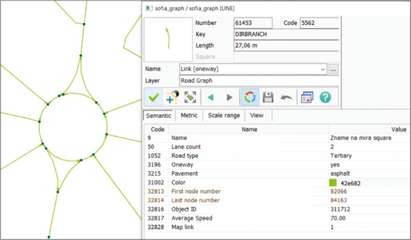
After the automated creation of the road graph, software topological graph control was performed. Its purpose is to determine whether the structure of the graph is correct − whether each edge has exactly two nodes corresponding to the connectivity matrix, whether there are no hanging nodes, intersection of edges without a node (if, of course, the edges are on the same level), and others. The result of this process is a correct graph structure of the research territory (Figure 1).

Figure 1. Segment of a Road graph, created from open-source data from OSM. / Slika 1. Segment cestovnog grafa, stvoren iz podataka otvorenog izvora iz OSM-a.
kig-22-66-g1.jpg

2.4. Georeferencing of road accident data from different sources according to ISO 19 148

When it comes to presenting networks in digital form and performing spatial analyzes on them, an indispensable element is the georeferencing of objects and events, considering the network structure, network limitations, the specificity of derivation, as well as the nature of the source data. One of the established methods in theory and practice is the so-called linear referencing – a method of data collection and location determination by using a measured distance along a linear object through the Linear Referencing System (LRS) (ISO 2012). The main applications are twofold (Scarponcini 2002) − performing linear segmentation of a section, thus allowing the dynamic nature of linear objects to be expressed, modeling their changing characteristics in different sections without dividing the object itself into separate parts, and georeferencing of an event. For the current development, the second application is of interest.

In order to perform the "spatial event referencing" task, a fundamental concept laid down in the linear referencing standard ISO 19 148 should be followed − to represent the location as a single position, 3 components are needed − a linear element that can be measured (for example by a graph structure with directed edges and defined weights), a linear method (absolute, relative or interpolative) and a measured value on the linear object (ISO 2012). However, such data are not always available, so the approach of georeferencing events and objects in practice is extended relative to the type of source data. For the physical performance of the task, as an element of the systematization of the data, functionalities have been introduced in the road accidents GIS in order that the final result is available regardless of the spatial indicator of the source data (absolute coordinates, address, mileage, relative location to a geographical object or other), and the end result is a standardized representation of the location of the event in accordance with international standardization.

3. Determination of Spatial Network Autocorrelation

Analyzing road accidents is a major task of road accidents GIS. The current development considers a specific case of defining a geographically oriented dependence between the number of road accidents in different locations considering the network nature of the transport system, namely − spatial network autocorrelation. General concepts in the field will be described, and then the physical determination of the autocorrelation coefficient for the regions of the Sofia City Municipality with real open-source road accident data, as well as its statistical reliability, will be presented step by step. For the physical implementation, an author's script was created with the capabilities of the Python programming language, which is implemented directly in the GIS Panorama console or as a separate application with a user interface.

3.1. Generalities of Spatial Network Autocorrelation

Spatial autocorrelation is known to be a correlation between attribute values of the same type at different locations (Odland 2020). A physical solution to this statistical method is presented by Moran with the so-called Moran's coefficient, or also found in the literature as Moran's I. Moran considers two cases − local (representing the correlation between the attribute values of a specific cell with those surrounding it) and global (representing the average local correlation between all cells) (Black 1992). The subject of analysis in the road accidents GIS is the local case, as it is more practically applicable, and it is also known that in the global case there is proportionality to the average value of all cells in the local case.

Practically, the autocorrelation coefficient indicates the presence or absence of linear dependence, and its value allows to characterize the strength of the relationship between the researched elements from the point of view of mathematical statistics. The goal of the analysis is the construction of a statistical model of dependence of the given indicator in each territorial unit and its neighboring units, considering the influence of selected factors. The presence of a statistical value of the autocorrelation coefficient indicates the occurrence of processes that determine the clustering of values in neighboring locations, and the addition of various factors in the model leads to an increase in the accuracy of statistical modeling (Eliseeva 2002,Samsonov 2022).

The network variety of the method involves determining a relationship between attribute values of edges of a network and similar values of other edges. This approach is used to achieve the objectives of the road accidents GIS, with the attribute values being the number of road accidents in administrative units.

A theoretical statement and various studies of the method can be found in (Anselin 1995,Black, Thomas 1998,Black 2010,Okabe, Sugihara 2012,Odland 2020,Samsonov 2022).

3.2. Steps to determine local spatial network autocorrelation

It is known that to perform a spatial network autocorrelation analysis, a set of edges and nodes, a set of attribute values, and a set of weight values are required. With this data available, several steps are performed to calculate it, following the sequence of actions defined in (Okabe, Sugihara 2012):

- Defining network space in a given territory. Such a space is defined for the territory of the city of Sofia, using open data from OSM, after which a correct topologically connected road graph is defined;

- Tessellating the network into non-overlapping and densely filling network cells. Here, the approach is used with a division by administrative units, accessible from open data and imported as polygon objects. Important attribute values are the system internal number (Number) and the OSM identifier, both values being unique (Figure 3, columns 5 and 2);

- Determination of representative points of the network. The main purpose of this step is the subsequent determination of spatial weights between territorial units. Here, the centers of the mass of the network cells are selected, and for each "region" polygon object, a centroid is generated by a built-in GIS algorithm. To account the network structure and the network constraints it imposes (such as one-way traffic for example), centroids are assigned to the corresponding nearest edge from the network using the shortest distance principle. An important element is the preservation of the connections between the generated centroids and the polygon objects, and this is done by means of internal keys, attached as an attribute value of the objects (Figure 3, column 7).

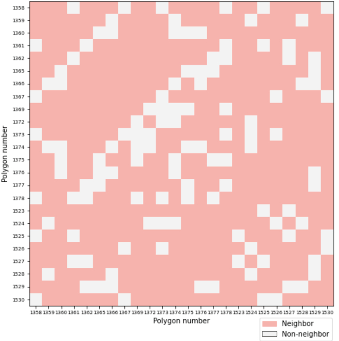
- Determining a neighborhood of the network cells. The goal is to define a neighborhood matrix to be used for subsequent calculations. For each polygon object, its neighbors are determined using a topological neighbor algorithm, also called the checkerboard method. The practical implementation is reduced to the determination of common points, and it is sufficient to determine even one point (Samsonov 2021). The method was used since it is suitable for territorial-administrative units for which it is certain that the topological connections are correct. For the practical implementation, a Python programming language script was created, through which the neighborhood is determined using the unique numbers of the polygon objects and their geometric position. The script sorts the polygons by number and creates adjacency links, as for non-adjacent polygons, the values are 0. The result is the so-called a binary neighborhood matrix (Figure 2) to be used to construct a spatial weights matrix.

After applying the neighborhood determination method, the identifiers of the neighboring polygon objects are added as an attribute of each region (Figure 3, column 4).

Figure 2. Binary topological neighborhood matrix resulting from the algorithm. / Slika 2. Binarna topološka matrica susjedstva.
kig-22-66-g2.jpg

- Calculation of spatial weights between all adjacent pairs of network cells. In general, the spatial weight characterizes the strength of the connection between territorial units, and the ordered set of all spatial weights is the well-known in theory weight matrix. The process of defining a weight matrix is defined by (Odland 2020) as one of the most important, as the weighting function is a means of ascertainment a hypothesis regarding relationships between the researched locations.

The development uses the metric weight defined in (Okabe, Sugihara 2012):

kig-22-66-g8.jpg

Where ds(pi, pj) is the shortest distance, and α and β are positive constants.

The used metric weight (1) is a function of the shortest distance on a network in the special case where the reciprocal of the distance in kilometers is used. In this model, the main idea is that closer objects have a greater influence on the result, which is practically an expression of the First Law of Geography, defined by (Tobler 2004) − "everything is connected to everything else, but nearby things are connected more than distant".

For each centroid (pre-assigned to its nearest edge), the shortest distance on network to all centroids of neighboring polygons is determined. Due to the presence of the neighborhood matrix, the computational resource is reduced by determining the distances only between neighboring cells and not between all.

The result of the physical execution through a Python script is a rectangular matrix of shortest distances with dimension the number of network cells, such that between non-adjacent cells, the values are 0. Based on the distances, spatial weights of each cell with each of its neighbors were calculated, using formula (1). The result is a weight matrix with dimension the number of polygon objects, again the relations of non-adjacent cells are assumed to be 0.

- Georeferencing of road accident data. This step aims to determine the total number of attribute values under analysis. With real road accident data available, each road accident can be georeferenced according to the linear reference standard depending on the availability of source data, and the result is a spatially defined object that is attached to a graph edge based on the shortest distance as needed.

The development used real data from an open data portal for road accidents [https://opendata.yurukov.net/], which contains spatial information about severe road accidents that occurred on the territory of the city of Sofia in KML format with an available text description. The data are processed by exporting the geodetic geographic coordinates and the available textual information. Structuring the data includes transforming the coordinates into the project coordinate system (the normatively established Bulgarian geodetic system BGS2005, UTM 35N, EPSG 7800), extracting the date from the textual data for its differentiation by query, adding the descriptive part as an attribute field and importing it in a GIS in a usable format. The available data contains 801 serious road accidents for 2013 and 487 for 2012.

Each road accident is assigned to a nearest edge automatically via a Python script, after which the total number of severe road accident for each area is determined.

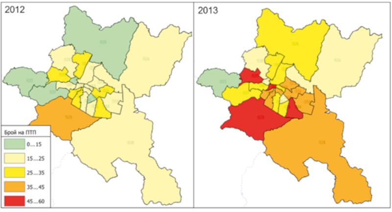
- Determining the total number of attribute values for each cell. The purpose of the step is to supply the last component necessary for calculating spatial autocorrelation – number of attribute data examined for each region. For each territorial unit, the number of serious road accidents within its boundaries is determined using a inner-point algorithm created in Python. The coordinates of the road accidents were used as an input parameter, and for each polygon object "region" it was determined whether the point is internal to its coordinates in the unified coordinate system. The result (number of accidents for each region) was assigned as an attribute value of each region (Figure 3, column 6,Figure 4) and it is used in the calculation of the autocorrelation.

Figure 3. Determining the number of road accidents for each territorial unit with output data from an open portal. / Slika 3. Utvrđivanje broja prometnih nesreća za svaku teritorijalnu jedinicu s izlaznim podatcima s otvorenog portala.
kig-22-66-g3.jpg

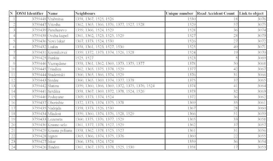
Figure 4. Thermically visualization − number of road accidents for 2012 and 2013. / Slika 4. Termička vizualizacija - broj prometnih nesreća za 2012. i 2013. godinu.
kig-22-66-g4.jpg

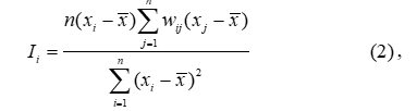
- Calculation of a local case of spatial autocorrelation by Moran's method. To determine the Moran index, the formulas from (Black, Thomas 1998,Black 2010,Anselin 1995) and (Okabe 2012) are used:

kig-22-66-g9.jpg

where: Ii autocorrelation Moran`s index;

n – number of polygon objects (territorial units);

xi – attribute value of the investigated indicator for current cell i;

kig-22-66-g10.jpg

is the empirical mathematical expectation, or the average value of the attributes for all network cells.

It should be noted that the index i denotes the current cell, and the index j denotes its neighboring cells. It is also assumed that ij and wii = 0.

The overall solution is performed using the built-in Python script, and the result is the determination of a Moran`s autocorrelation index value for each territorial unit (Figure 5, column 3). For code efficiency, the denominator is only considered once since it is a constant value.

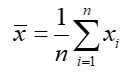
- Assessment of the accuracy and reliability of the autocorrelation coefficient. Typically, the null hypothesis approach is used to assess accuracy, in which a comparison is made with a variable assumed to be normally distributed (Anselin 1995,Okabe 2012, Samsonov 2020). The null hypothesis states that the analyzed variables are randomly and independently distributed in the studied territories.

The formulas from (Black, Thomas 1998,Black 2010,Anselin 1995,Okabe 2012,Leung et al. 2003s) are used to estimate the accuracy:

kig-22-66-g11.jpg

where: E(Ii) – theoretical expected value;

wij – weighting coefficients from a weighting matrix;

n – number of all network cells;

D(Ii) – variance of the coefficient.

The variance formula is derived in (Leung et al. 2003) and (Anselin 1995).

The physical meaning of the theoretical expected value is that if the empirically determined value of the coefficient approaches it within the limits of the statistical confidence probability, the values of the studied variable are independent with respect to the neighboring locations. As can be seen from the formula (3), the expected value is a function of the weighting coefficients and the number of studied areas and does not depend on the studied variable. Values that exceed more than 3 times the standard deviation (the so-called rule of three sigma) indicate positive spatial autocorrelation, and values that are 3 times below it indicate negative autocorrelation (Odland 2020).

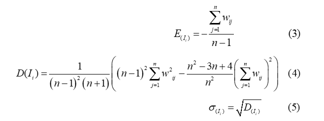
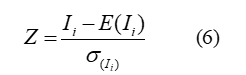
Indicators of "significance" are the z-value and corresponding to each z-value probability or p-value of the coefficient (Samsonov 2020):

kig-22-66-g12.jpg

The described formulas are algorithmized using the Python programming language, and a list of Laplace coefficients is created for Fisher's criterion. The results of the calculations, representing the accuracy and reliability of the coefficient, are assigned as attribute values to the "region" objects. For graphical presentation, the hypsometric thematic visualization with the autocorrelation index is used (Figure 6).

Figure 5a. Presentation of Moran's coefficient for spatial autocorrelation of road accidents and its assessment of accuracy and reliability as an attribute value of regions of Sofia for 2012. / Slika 5a. Prikaz Moranova koeficijenta za prostornu autokorelaciju prometnih nesreća i njegove procjene točnosti i pouzdanosti kao vrijednosti atributa regija Sofije za 2012. godinu.
kig-22-66-g5.jpg

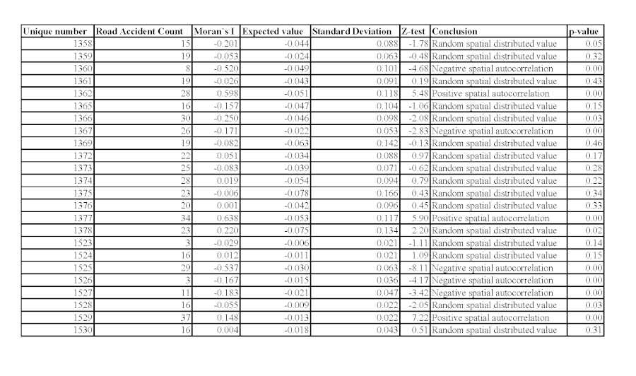
Figure 5b. Presentation of Moran's coefficient for spatial autocorrelation of road accidents and its assessment of accuracy and reliability as an attribute value of regions of Sofia for 2013. / Slika 5b. Prikaz Moranova koeficijenta za prostornu autokorelaciju prometnih nesreća i njegove procjene točnosti i pouzdanosti kao vrijednosti atributa regija Sofije za 2013. godinu.
kig-22-66-g7.jpg

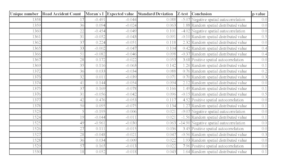
Figure 6. Hypsometric thematic visualization of spatial autocorrelation of road accidents in Sofia Municipality for 2012 and 2013. / Slika 6. Hipsometrijska tematska vizualizacija prostorne autokorelacije prometnih nesreća u općini Sofija za 2012. i 2013. godinu.
kig-22-66-g6.jpg

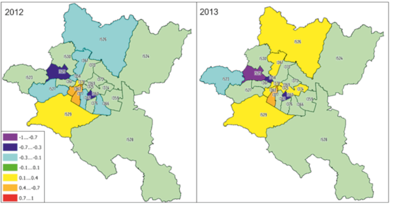
- Interpretation of the results. For the interpretation of the results, the statement of (Anselin 1995) can be used that positive values of the index (with reliability according to the rule of three sigma) inform about spatial clustering of similar values (high or low), and negative values of the index − about clustering of dissimilar values (for example, an area of high values surrounded by areas of low values). It should be noted that, of course, the values of the autocorrelation coefficient depend on the chosen weighting model. In this case, a different from the standard binary model was chosen, which reflects only the presence or absence of contiguity.

The analysis of the results determines that for 5 regions out of 24 for both years there is the presence of spatial autocorrelation with z-value >1.96 and correspondingly p-value <0.05. The regions with established autocorrelation are: 1377 with a strongly pronounced positive for both years −0.43 and 0.68, respectively; and 1529 with a weak positive for both years −0.15 and 0.17, respectively. The two regions are adjacent, i.e. a clustering indicator with common metrics is available. A factor in the availability of the index is the claim that the two regions have a similar number of road accidents as the neighboring locations. For region 1360 and 1525, a clearly expressed negative spatial correlation is established for both years (respectively −0.52 and −0.45 and −0.53 and −0.96). A factor in this result is the fact that in 1360 there are more than twice as many road accidents compared to the surrounding areas, and in 1525 more than twice as many road accidents as compared to those surroundings it. For the region 1358 in both years there was once a randomness with a confidence probability of the limit (95%), once a strong negative value, and this can be interpreted as two consecutive years with a negative autocorrelation with a risk of error of 5%. This negative index shows that there is a noticeable difference in the number of road accidents with the neighboring regions. A similar approach can be applied to region 1362. These spatial results can be used to determine the so-called "black areas" with a concentration of traffic accidents and as a foundation for subsequent analysis of various factors to establish complex of causes for the autocorrelation index values.

In more than 50% of the regions, both consecutive years show that there is no spatial autocorrelation, therefore it can be assumed that the number of road accidents in them is distributed randomly and independently of the neighboring locations. In three of the regions, there is a variation between a positive and a negative coefficient for both years, with the coefficient having a small value <0.2 (this are 1367, 1526 and 1527). Given the small value of the coefficient, various hypotheses can be made with the subject of subsequent analysis.

The above statements are with a degree of reliability calculated as the last component of the development (Figure 5, columns 4, 5, 6, 7 and 8). Here, the fundamental rule in mathematical statistics should be considered, that the absolute value of the coefficient is not of primary importance, but its degree of accuracy and reliability, which is a fact of the results.

As with any spatial statistical model, the interpretation of the results is a function of the accuracy, reliability, and completeness of the source data. It should be noted that the data is archival (from 2012 and 2013), and its completeness and veracity are not guaranteed by its source. Also, the studied areas are of different area. In this regard, considering the dynamics in the management of the transport system, the results of their analysis are also not of a sufficient degree of relevance, which is the reason of not carrying out in-depth analysis. The main goal of the research is to demonstrate a methodology for performing spatial analysis of road accidents.

4. Conclusion and Suggestions for Further Work

As a general conclusion, a methodology for representing a road network through a graph and determining a spatial network autocorrelation index of road accidents on it can be summarized to spatially analyze various events, and in particular road accidents.

The result can be considered in two aspects − the realization of a pilot project for spatially analyzing events through the spatial autocorrelation model on a network, which is at a degree of completion sufficient to be implemented in the analysis of road accidents; and the appeal to take action to provide access to spatially defined open data in a sphere as strategically important as transport and related road accidents on the territory of the Republic of Bulgaria as an element of reducing traffic injuries.

As a future development, an examination of event values with different weight models, a function of heterogeneous parameters, can be performed, thereby discovering useful relationships. As a research element, the accuracy estimation setup can be extended, and hypotheses tested for different types of distributions to evaluate the result more objectively. Time can also be added as a component of the analysis. Also, analyzes can be presented through various types of graphics and implemented in a web-based application, such as a GIS Web Server, to access information from a wide range of users, as well as update information in near real-time from various sources, including from the institutions managing the transport. The functionalities of the system provide an opportunity to manage and publish in near real-time, including periodic automated analysis of information about road accidents and other events. As a result, using GIS web-services (such as WFS, WMS and others), all products and services can be freely accessed.


1. Uvod

Složeno geografski orijentirano modeliranje u području prometa, uključujući modeliranje elemenata cestovne infrastrukture, povezanih prostornih događaja, kao i statističko-matematičko modeliranje ovisnosti među njima, predstavlja izazov kada je u pitanju rješavanje više zadataka. Suvremeni pristup modeliranju uključuje primjenu logike međunarodne normizacije u geoinformacijskim izvorima. Slijedeći ideju sinergije, jednom stvoren na temelju konceptualnog modela (Kunchev, Angelova 2023), fizički je model cestovne infrastrukture kao element geoinformacijskog sustava (GIS) multifunkcionalan – može služiti ne samo za logističke zadatke, već i za prikladnu ocjenu stanja površina i objekata ceste i uz ceste, identifikaciju problematičnih područja, kao i naravno, za analizu svih vrsta procesa koji se događaju na prometnoj infrastrukturi ili blizu nje.

U tako širokom području kao što su promet i prometne nesreće, mnogobrojne su primjene digitalnog modela cestovne infrastrukture i moguće analize. Istraživanje je usmjereno na definiranje ispravnih temelja za analizu s pomoću digitalnog modela ceste, temeljenog na podatcima otvorenog koda; izradu cestovnog grafa s naglaskom na potrebe i probleme u njegovoj izradi; sistematizaciju i georeferenciranje događaja (osobito prometnih nesreća) na temelju međunarodnih normi za linearno referenciranje i primjenu jednog od mnogobrojnih algoritama za analizu prometnih nesreća − prostorna autokorelacija s odrazom mrežne prirode cesta, kao i evaluacija rezultata analize s dokazanim matematičkim pristupima. Opisani procesi, realizirani fizički za područje grada Sofije s otvorenim podatcima s geoportala OpenStreetMap (OSM) i softverskim mogućnostima GIS Panorama i programskog jezika Python, bit će uzeti u obzir.

Važna je studija na temu digitalnog modela cesta (Demidenko, el al. 2020), gdje se koncept inteligentnog prometnog sustava razmatra kao skup usluga integriranih u jedinstveni geoinformacijski prostor, s naglaskom na fizičkom vektorskom prikazu cestovnog grafa. Temeljna su postignuća u području analize prometnih nesreća kroz prostornu autokorelaciju (Anselin 1995), gdje je uvedena statistička metoda za lokalne pokazatelje prostorne autokorelacije, postavljeni temelji analize i pristup praktično ispitan studijom nacionalnih sukoba u zemljama Afrike (Black 2010), gdje se uvodi mrežna prostorna autokorelacija, predstavlja pristup smanjenju njezinog utjecaja modeliranjem, s naglaskom na činjenicu da je to matematički ekvivalent obične statističke varijante s razlikom u mrežnoj strukturi i s njom povezanim težinama (Black, Thomas 1998), gdje se utvrđuju čimbenici koji karakteriziraju tzv. "crne zone" podložni grupiranju koje se može uspostaviti razmatranim pristupom. Ključna su dostignuća u vezi s procjenom točnosti koeficijenta autokorelacije (Samsonov 2021), gdje se algoritamski detaljno razmatraju računanja i vizualizacije rezultata te (Valchinov, Kostadinov 2012) gdje su postavljeni statistički temelji korelacijskog koeficijenta.

2. Definiranje ispravne osnove za analizu prostorne mreže s pomoću digitalnog modela cesta

Prema jedinstvenom pristupu niza normi koje se bave prostornim informacijama ISO/TC 211 − Geografske informacije/Geomatika, modeliranje geoprostornih proizvoda, procesa i usluga prikazano je na četiri razine – meta-metamodel, metamodel, razina aplikacije i fizička razina (Govorov 2008,Kunchev 2023). Nakon što su provedena prva tri koraka u (Lipiyska, Angelova 2020,Kunchev, Angelova 2023) i (Angelova 2023), četvrti će se razmotriti, jer njegov je element definicija ispravne osnove za potrebe potpunog GIS-a prometnih nesreća.

Važno je uvesti koncept digitalnog modela ceste (DMC) kao skupa informacijskih izvora, uključujući digitalne informacije o objektima prometnog sustava, prometnim uvjetima i graf cestovne mreže (Demidenko et al. 2020). Taj se koncept upotrebljava kao polazište prilikom definiranja temelja za glavnu svrhu GIS-a prometnih nesreća − analizu događaja s ciljem smanjenja ozljeda u prometu.

Razmotrit će se pojedinačne komponente za postizanje konačnog cilja − pristup, kontrola unosa i sistematizacija otvorenih podataka, izrada cestovnog grafa s dovoljnom razinom detalja za ispravan prijenos informacija o prometnim nesrećama, georeferenciranje događaja i postupak njihove dodjele mreži na temelju međunarodne normizacije u tom području.

2.1. Pristup otvorenim podatcima − određivanje opsega, filtriranje, sistematizacija i kontrola unosa

Upotrijebljena su dva glavna skupa vektorskih podataka otvorenog koda s geoportala OSM − prvi predstavlja različite klase cesta unutar odabranog područja s dostupnim informacijama o atributima, a drugi − najmanje dostupne teritorijalne jedinice za područje grada Sofije u OSM-u − regije općine grada Sofije. Jedan od kriterija po kojem su odabrane regije općine činjenica je da se njihove granice poklapaju s cestovnim prometnicama proučavanog područja.

Podatcima se pristupilo i povezalo ih upitom, eksportiralo u jedan od formata za razmjenu prostornih podataka − GeoJSON, a zatim učitalo u GIS Panorama. Kako bi bili maksimalno iskoristivi, podatci su sistematizirani, uz naznaku podudarnosti između objekata iz datoteke GeoJSON i specijaliziranog klasifikatora kreiranog za potrebe rada s otvorenim podatcima iz izvora OSM. Taj je proces detaljno razmatrala (Angelova 2023). Korištenje klasifikatora cesta također se može smatrati elementom kontrole unosa podataka − to je mjesto za provjeru podudaranja tipova podataka atributa, utvrđivanje prisutnosti/odsutnosti obveznih podataka i metapodataka, provjeru jedinstvenosti identifikatora vanjskog sustava, kao i stvaranje nekih internih i drugih.

2.2. Topološka povezanost ulaznih podataka

Rad s bilo kojom vrstom vektorskih podataka zahtijeva topološki integritet, tj. izradu topološkog modela za organiziranje prostornih odnosa između značajki (Pavlov, Dechev 2016). Nakon sistematizacije i provjere atributa podataka potrebno je izvršiti i metričku provjeru. Prije izrade cestovnog grafa izvršena je softverska kontrola metričkih podataka na različitim vrstama cesta, koje su vektorski objekti.

Kada se radi s različitim vrstama vektorskih podataka (poligoni, linija, točka), dostupni su mnogi parametri koji se mogu provjeriti i prilagoditi, kao što su zatvaranje i nepreklapanje poligonskih objekata, prisutnost krajnjih točaka, unutrašnjost poligonskih objekata, duplikati objekata i drugo (ArcGIS 2010). Prilikom kontrole linearnih objekata, glavne su komponente provjera povezanosti unutar određenog dopuštenog odstupanja (tolerancije) i prisutnost objekata premale duljine, koji su općenito parazitski. U konkretnom slučaju za područje grada Sofije, s obzirom da su podatci otvorenog izvora, otkrivene su i ispravljene 3 metričke pogreške − 2 objekta premale duljine i 1 dupliranje točke u jednom linearnom segmentu.

2.3. Izrada cestovnog grafa − zahtjevi ovisno o ciljevima, problemi pri izradi i njihovo rješenje

Nakon što je kroz osnovne korake kontrole unosa provjerena topologija i povezanost atributa mreže, sljedeći je korak izrada cestovnog grafa kao elementa DMC-a za područje Sofije. U tu je svrhu upotrijebljena softverska komponenta za izradu strukture grafa s ulaznim parametrom pet glavnih klasa cestovne mreže dostupnih iz OSM-a, s ukupnim brojem objekata od 34 700. U izradi grafa upotrijebljen je specijalizirani klasifikator prilagođen potrebama cestovnog grafa koji sadrži potrebne komponente, kao što su rubovi, čvorovi, smjer prikazan strelicama i drugo. Naravno, dostupni su podatci o atributima i vizualni prikaz.

Algoritmizacija uključuje važne parametre, uključujući, između ostalog:

  • semantiku iz koje se izvodi prisutnost jednosmjernog prometa;

  • ograničenje brzine na različitim vrstama cesta. Ovdje je dostupna mogućnost izvođenja brzine iz semantike, ali u OSM-u otvorenog koda nema takvih informacija za svaku dionicu ceste, pa je odabran pristup generalizacije prema tipovima cesta. Taj pristup ne uzima u obzir lokalna ograničenja brzine koja su uvedena prometnim znakovima, no treba napomenuti da ako su dostupni detaljniji podatci o dionicama, oni se mogu upotrijebiti za poboljšanje točnosti;

  • semantiku koja se dodjeljuje na rubovima grafa. Ključna je komponenta u definiranju grafa dodjela njegovim rubovima karakteristika koje se odnose na stvarne cestovne objekte. U tom se slučaju biraju naziv, smjer, kolnik, broj prometnih traka, opis ograničenja i širina. Mogu se odabrati sve dostupne značajke, no opet se vodilo računa o dostupnosti i potpunosti izvornih podataka;

  • održavanje veze s digitalnom kartom. Važna je komponenta održavanje odnosa između podataka grafa i izvornih podataka. To je pitanje kojim se bavi međunarodna normizacija, točnije norma ISO 19 148 – Geoinformacije – Linearno referenciranje (ISO 2012). Norma definira da se u mrežnom prikazu topološki aspekt jasno razlikuje od skupa prostornih podataka i njegovog kartografskog prikaza te je sadržan u strukturi grafa čvorova i rubova. Taj se pristup upotrebljava i za pojednostavljenje računanja i uklanjanje potrebe za upotrebom velike veličine prostornih podataka, te kada je potrebna dinamička segmentacija s različitim parametrima, kao što su kolnik, ograničenje brzine, broj traka i drugi (INSPIRE tematska radna skupina Prometne mreže 2014). Povezanost grafa s digitalnom kartom omogućena je softverskom opcijom "zadrži vezu s kartom", čiji je princip dodjela internog identifikatora ili jedinstvenog identifikatora OSM-a semantici rubova.

Nakon automatizirane izrade cestovnog grafa izvršena je softverska topološka kontrola grafa. Svrha mu je utvrditi je li struktura grafa ispravna − ima li svaki rub točno dva čvora koja odgovaraju matrici povezanosti, nema li visećih čvorova, sjecišta rubova bez čvora (ako su, naravno, rubovi na istoj razini) i drugo. Rezultat je tog procesa ispravna struktura grafa područja istraživanja (slika 1).

2.4. Georeferenciranje podataka o prometnim nesrećama iz različitih izvora u skladu s normom ISO 19 148

Kada je u pitanju prikaz mreža u digitalnom obliku i izvođenje prostornih analiza na njima, neizbježan je element georeferenciranje objekata i događaja, imajući u vidu strukturu mreže, ograničenja mreže, specifičnosti derivacije, kao i prirodu izvornih podataka. Jedna od etabliranih metoda u teoriji i praksi je tzv. linearno referenciranje – metoda prikupljanja podataka i određivanja lokacije s pomoću izmjerene udaljenosti uzduž linearnog objekta putem sustava linearnog referenciranja (SLR) (ISO 2012). Glavne su primjene dvojake (Scarponcini 2002) − izvođenje linearne segmentacije dijela, čime se omogućuje izražavanje dinamičke prirode linearnih objekata, modeliranje njihovih promjenjivih karakteristika u različitim dijelovima bez dijeljenja samog objekta na zasebne dijelove i georeferenciranje događaja. Za trenutni razvoj zanimljiva je druga primjena.

Kako bi se izvršio zadatak "referenciranja prostornog događaja", treba se pridržavati temeljnog koncepta određenog u normi linearnog referenciranja ISO 19 148 − da bi se lokacija predstavila kao jedna pozicija, potrebne su 3 komponente − linearni element koji se može izmjeriti (primjerice strukturom grafikona s usmjerenim rubovima i definiranim težinama), linearnom metodom (apsolutnom, relativnom ili interpoliranom) i izmjerenom vrijednošću na linearnom objektu (ISO 2012). Međutim, takvi podatci nisu uvijek dostupni, pa se pristup georeferenciranju događaja i objekata u praksi proširuje u odnosu na vrstu izvornih podataka. Za fizičku izvedbu zadatka, kao element sistematizacije podataka, u GIS-u prometnih nesreća uvedene su funkcionalnosti kako bi konačni rezultat bio dostupan bez obzira na prostorni pokazatelj izvornih podataka (apsolutne koordinate, adresa, kilometraža, relativna lokacija u odnosu na geografski objekt ili drugo), a krajnji je rezultat standardizirani prikaz lokacije događaja u skladu s međunarodnom normizacijom.

3. Određivanje autokorelacije prostorne mreže

Analiza prometnih nesreća glavna je zadaća GIS-a prometnih nesreća. Trenutačni razvoj razmatra specifičan slučaj definiranja geografski orijentirane ovisnosti između broja prometnih nesreća na različitim lokacijama s obzirom na mrežnu prirodu prometnog sustava, odnosno − autokorelaciju prostorne mreže. Opisat će se opći koncepti u tom području, a potom će se korak po korak predstaviti fizičko određivanje koeficijenta autokorelacije za regije općine grada Sofije sa stvarnim podatcima o prometnim nesrećama otvorenog koda, kao i njegova statistička pouzdanost. Za fizičku primjenu izrađena je autorska skripta s mogućnostima programskog jezika Python koja se učita izravno u konzolu GIS-a Panorama ili kao zasebna aplikacija s korisničkim sučeljem.

3.1. Općenite napomene o autokorelaciji prostorne mreže

Poznato je da je prostorna autokorelacija korelacija između vrijednosti atributa iste vrste na različitim lokacijama (Odland 2020). Moran je fizičko rješenje te statističke metode predstavio takozvanim Moranovim koeficijentom, koji se u literaturi nalazi i kao Moranov I. Moran razmatra dva slučaja − lokalni (predstavlja korelaciju između vrijednosti atributa određene ćelije s onima koje je okružuju) i globalni (predstavlja prosječnu lokalnu korelaciju između svih ćelija) (Black 1992). Predmet je analize u GIS-u prometnih nesreća lokalni slučaj, jer je praktičniji za primjenu, a poznato je i da u globalnom slučaju postoji proporcionalnost s prosječnom vrijednosti svih ćelija u lokalnom slučaju.

Praktično, koeficijent autokorelacije ukazuje na prisutnost ili odsutnost linearne ovisnosti, a njegova vrijednost omogućuje karakterizaciju snage odnosa između istraživanih elemenata sa stajališta matematičke statistike. Cilj je analize konstrukcija statističkog modela ovisnosti zadanog pokazatelja u svakoj teritorijalnoj jedinici i njenim susjednim jedinicama, uzimajući u obzir utjecaj odabranih čimbenika. Prisutnost statističke vrijednosti koeficijenta autokorelacije ukazuje na pojavu procesa koji određuju grupiranje vrijednosti na susjednim lokacijama, a dodavanje različitih čimbenika u model dovodi do povećanja točnosti statističkog modeliranja (Eliseeva 2002,Samsonov 2022).

Vrsta mreže metode uključuje određivanje odnosa između vrijednosti atributa rubova mreže i sličnih vrijednosti drugih rubova. Tim se pristupom ostvaruju ciljevi GIS-a prometnih nesreća, a vrijednosti su atributa broj prometnih nesreća u administrativnim jedinicama.

Teorije o tome i različite studije mogu se pronaći u literaturi (Anselin 1995,Black, Thomas 1998,Black 2010,Okabe, Sugihara 2012,Odland 2020,Eliseeva 2002,Samsonov 2022).

3.2. Koraci za određivanje autokorelacije lokalne prostorne mreže

Poznato je da je za izvođenje analize autokorelacije prostorne mreže potreban skup rubova i čvorova, skup vrijednosti atributa i skup vrijednosti težina. S tim dostupnim podatcima, izvodi se nekoliko koraka za njihovo računanje, prateći slijed radnji definiranih u (Okabe, Sugihara 2012):

- Definiranje mrežnog prostora na određenom teritoriju. Takav je prostor definiran za područje Sofije, koristeći otvorene podatke iz OSM-a, nakon čega je definiran točan topološki povezan cestovni graf;

- Teseliranje mreže u mrežne ćelije koje se ne preklapaju i gusto ispunjavaju. Ovdje se upotrebljava pristup s podjelom po administrativnim jedinicama, dostupnom iz otvorenih podataka i uvezenim kao poligonski objekti. Važne su vrijednosti atributa interni broj sustava (Number) i identifikator OSM-a, pri čemu su obje vrijednosti jedinstvene (slika 3, stupci 5 i 2);

- Određivanje reprezentativnih točaka mreže. Glavna je svrha ovog koraka naknadno određivanje prostornih težina između teritorijalnih jedinica. Ovdje se odabiru središta mase mrežnih ćelija, a za svaki se poligonski objekt "regije" ugrađenim GIS-algoritmom generira središte mase. Kako bi se uzela u obzir mrežna struktura i mrežna ograničenja koja ona nameće (primjerice, jednosmjerni promet), centroidi se dodjeljuju odgovarajućem najbližem rubu mreže upotrebom načela najkraće udaljenosti. Važan je element očuvanje veza između generiranih centroida i poligonskih objekata, a to se postiže pomoću internih ključeva, priloženih kao vrijednost atributa objekata (slika 3, stupac 7).

- Određivanje susjedstva mrežnih ćelija. Cilj je definirati matricu susjedstva koja će se koristiti za naknadna računanja. Za svaki poligonski objekt, njegovi se susjedi određuju s pomoću topološkog algoritma susjeda, koji se zove i metoda šahovnice. Praktična provedba svodi se na određivanje zajedničkih točaka, a dovoljno je odrediti i samo jednu točku (Samsonov 2021). Ta je metoda upotrebljena jer je prikladna za teritorijalno-administrativne jedinice za koje je sigurno da su topološke veze ispravne. Za praktičnu provedbu izrađena je skripta u programskom jeziku Python s pomoću koje se susjedstvo određuje s pomoću jedinstvenih brojeva poligonskih objekata i njihovih geometrijskih položaja. Skripta sortira poligone prema broju i stvara veze susjedstva, jer za nesusjedne poligone vrijednosti su 0. Rezultat je takozvana binarna matrica susjedstva (slika 2) koja se upotrebljava za konstrukciju matrice prostornih težina.

Nakon primjene metode određivanja susjedstva dodaju se identifikatori susjednih poligonskih objekata kao atributi svake regije (slika 3, stupac 4).

- Računanje prostornih težina između svih susjednih parova mrežnih ćelija. Općenito, prostorna težina karakterizira snagu povezanosti između teritorijalnih jedinica, a uređeni je skup svih prostornih težina u teoriji dobro poznata matrica težine. Proces definiranja matrice težine definiraOdland (2020) kao jedan od najvažnijih, jer je funkcija težine sredstvo utvrđivanja hipoteze o odnosima između istraživanih lokacija.

U radu se koristi metrička težina definiranu u (Okabe, Sugihara 2012):

kig-22-66-g8.jpg

gdje je ds(pi, pj) najkraća udaljenost, a α i β pozitivne konstante.

Upotrijebljena metrička težina (1) funkcija je najkraće udaljenosti na mreži u posebnom slučaju kada se koristi recipročna vrijednost udaljenosti u kilometrima. U ovom modelu, glavna je ideja da bliži objekti imaju veći utjecaj na rezultat, što je praktički izraz Prvog zakona geografije, koji definira (Tobler 2004) - "sve je povezano sa svim ostalim, ali stvari koje su bliže povezane su više nego udaljene".

Za svaki se centroid (unaprijed dodijeljen njegovom najbližem rubu) određuje najkraća udaljenost na mreži do svih centroida susjednih poligona. Zbog prisutnosti matrice susjedstva računalni se resurs smanjuje određivanjem udaljenosti samo između susjednih ćelija, a ne između svih.

Rezultat fizičkog izvođenja s pomoću Pythona pravokutna je matrica najkraćih udaljenosti s dimenzijom broja mrežnih ćelija, tako da je između nesusjednih ćelija vrijednosti 0. Na temelju udaljenosti, s pomoću formule (1) izračunane su prostorne težine svake ćelije sa svakim od njenih susjeda. Rezultat je matrica težine s dimenzijom broja poligonskih objekata, a ponovno se pretpostavlja da su odnosi nesusjednih ćelija 0.

The result of the physical execution through a Python script is a rectangular matrix of shortest distances with dimension the number of network cells, such that between non-adjacent cells, the values are 0. Based on the distances, spatial weights of each cell with each of its neighbors were calculated, using formula (1). The result is a weight matrix with dimension the number of polygon objects, again the relations of non-adjacent cells are assumed to be 0.

- Georeferenciranje podataka o prometnim nesrećama. Taj korak ima za cilj odrediti ukupan broj vrijednosti atributa koji se analiziraju. S dostupnim podatcima o stvarnim prometnim nesrećama, svaka se prometna nesreća može georeferencirati prema linearnom referentnom standardu ovisno o dostupnosti izvornih podataka, a rezultat je prostorno definiran objekt koji je pridružen po potrebi rubu grafa na temelju najkraće udaljenosti.

U radu su se koristili stvarni podatci s portala otvorenih podataka za prometne nesreće [https://opendata.yurukov.net/], koji sadrži prostorne informacije o teškim prometnim nesrećama koje su se dogodile na području Sofije u formatu KML s dostupnim tekstualnim opisom. Podatci su obrađeni izvozom geodetskih geografskih koordinata i dostupnih tekstualnih informacija. Strukturiranje podataka uključuje transformaciju koordinata u koordinatni sustav projekcije (normativno uspostavljeni bugarski geodetski sustav BGS2005, UTM 35N, EPSG 7800), izdvajanje datuma iz tekstualnih podataka radi njegove diferencijacije upitom, dodavanje opisnog dijela kao polja atributa i uvozeći ga u GIS u upotrebljivom formatu. Dostupni podatci sadrže 801 tešku prometnu nesreću za 2013. godinu i 487 za 2012. godinu.

Svaka se prometna nesreća automatski dodjeljuje najbližem rubu putem skripte u Pythonu, nakon čega se utvrđuje ukupan broj teških prometnih nesreća za svako područje.

- Određivanje ukupnog broja vrijednosti atributa za svaku ćeliju. Svrha je ovog koraka osigurati posljednju komponentu potrebnu za računanje prostorne autokorelacije – broj ispitanih podataka atributa za svaku regiju. Za svaku teritorijalnu jedinicu broj se teških prometnih nesreća unutar njezinih granica utvrđuje s pomoću algoritma unutarnje točke kreiranog u Pythonu. Kao ulazni parametar upotrijebljene su koordinate prometnih nesreća, a za svaku „regiju" poligonskog objekta utvrđeno je je li točka interna svojim koordinatama u jedinstvenom koordinatnom sustavu. Rezultat (broj nesreća za svaku regiju) dodijeljen je kao vrijednost atributa svake regije (slika 3, stupac 6,slika 4) i upotrijebljen je u računanju autokorelacije.

- Računanje lokalnog slučaja prostorne autokorelacije Moranovom metodom. Za određivanje Moranovog indeksa upotrijebljene su formule iz (Black, Thomas 1998,Black 2010,Anselin 1995) i (Okabe 2012):

kig-22-66-g9.jpg

pa je: Ii Moranov indeks autokorelacije;

n – broj poligonskih objekata (teritorijalnih jedinica);

xi – vrijednost atributa ispitivanog indikatora za aktualnu ćeliju i;

kig-22-66-g10.jpg

empirijsko matematičko očekivanje, odnosno prosječna vrijednost atributa za sve mrežne ćelije.

Treba napomenuti da indeks i označava aktualnu ćeliju, a indeks j označava njezine susjedne ćelije. Također se pretpostavlja da je ij i wii = 0.

Cjelokupno rješenje provodi se s pomoću ugrađene skripte u Python, a rezultat je određivanje vrijednosti Moranovog indeksa autokorelacije za svaku teritorijalnu jedinicu (slika 5, stupac 3). Za učinkovitost se koda nazivnik uzima u obzir samo jednom jer je konstantna vrijednost.

- Procjena točnosti i pouzdanosti koeficijenta autokorelacije. Obično se za procjenu točnosti upotrebljava pristup nul-hipoteze, u kojem se uspoređuje s varijablom za koju se pretpostavlja da je normalno raspodijeljena (Anselin 1995,Okabe 2012, Samsonov 2020). Nul-hipoteza kaže da su analizirane varijable nasumično i neovisno raspoređene po istraživanim teritorijima.

Formule iz (Black, Thomas 1998,Black 2010,Anselin 1995,Okabe 2012,Leung i dr. 2003) upotrijebljene su za procjenu točnosti:

kig-22-66-g11.jpg

pa je: E(Ii) – teorijska očekivana vrijednost;

wij – težinski koeficijenti iz težinske matrice;

n – broj svih mrežnih ćelija;

D(Ii) – varijanca koeficijenta.

Formula varijance izvedena je u (Leung i dr. 2003) i (Anselin 1995).

Fizičko je značenje teorijske očekivane vrijednosti da ako joj se empirijski određena vrijednost koeficijenta približava u granicama pouzdanosti statističke vjerojatnosti, vrijednosti proučavane varijable neovisne su u odnosu na susjedne lokacije. Kao što je vidljivo iz formule (3), očekivana je vrijednost funkcija težinskih koeficijenata i broja proučavanih područja i ne ovisi o proučavanoj varijabli. Vrijednosti koje prelaze više od 3 puta standardnu devijaciju (tzv. pravilo tri sigme) označavaju pozitivnu prostornu autokorelaciju, a vrijednosti koje su 3 puta ispod nje označavaju negativnu autokorelaciju (Odland 2020).

Pokazatelji su "značajnosti" z-vrijednost i odgovarajuća vjerojatnost z-vrijednosti ili p-vrijednost koeficijenta (Samsonov 2020):

kig-22-66-g12.jpg

Opisane formule programirane su s pomoću Pythona, a za Fisherov kriterij kreiran je popis Laplaceovih koeficijenata. Rezultati računanja, koji predstavljaju točnost i pouzdanost koeficijenta, dodjeljuju se kao vrijednosti atributa objektima "regije". Za grafički se prikaz upotrebljava hipsometrijska tematska vizualizacija s indeksom autokorelacije (slika 6).

- Tumačenje rezultata. Za tumačenje rezultata može se upotrijebiti tvrdnjaAnselina (1995) da pozitivne vrijednosti indeksa (s pouzdanošću u skladu s pravilom tri sigme) govore o prostornom grupiranju sličnih vrijednosti (visokih ili niskih), a negativne vrijednosti indeksa − o grupiranju različitih vrijednosti (na primjer, područje visokih vrijednosti okruženo područjima niskih vrijednosti). Treba napomenuti da vrijednosti koeficijenta autokorelacije, naravno, ovise o odabranom modelu ponderiranja. U ovom je slučaju odabran drugačiji od standardnog binarnog modela, koji odražava samo prisutnost ili odsutnost kontiguiteta.

Analizom je rezultata utvrđeno da za 5 od 24 regija za obje godine postoji prostorna autokorelacija sa z-vrijednošću >1,96 i odgovarajućom p-vrijednošću <0,05. Regije s uspostavljenom autokorelacijom su: 1377 s jako izraženom pozitivom za obje godine −0,43 odnosno 0,68; i 1529 sa slabom pozitivom za obje godine −0,15 odnosno 0,17. Te su dvije regije susjedne, tj. dostupan je indikator klasteriranja sa zajedničkim metričkim vrijednostima. Čimbenik dostupnosti indeksa tvrdnja je da te dvije regije imaju sličan broj prometnih nesreća kao i susjedne lokacije. Za regiju 1360 i 1525 utvrđena je jasno izražena negativna prostorna korelacija za obje godine (−0,52 i −0,45, odnosno −0,53 i −0,96). Faktor takvog rezultata činjenica je da je u 1360 više nego dvostruko više prometnih nesreća u odnosu na okolna područja, a u 1525 više nego dvostruko više prometnih nesreća u odnosu na okolna područja. Za regiju 1358 u obje godine jednom je postojala slučajnost s vjerojatnošću pouzdanosti granice (95%), jednom jaka negativna vrijednost, a to se može protumačiti kao dvije uzastopne godine s negativnom autokorelacijom s rizikom pogreške od 5%. Taj negativni indeks pokazuje da postoji primjetna razlika u broju prometnih nesreća sa susjednim regijama. Sličan se pristup može primijeniti na regiju 1362. Ti se prostorni rezultati mogu upotrebljavati za određivanje tzv. "crnih područja" s koncentracijom prometnih nesreća i kao temelj za naknadnu analizu različitih čimbenika za utvrđivanje kompleksa uzroka vrijednosti indeksa autokorelacije.

U više od 50% regija obje uzastopne godine pokazuju da ne postoji prostorna autokorelacija, stoga se može pretpostaviti da je broj prometnih nesreća u njima raspoređen nasumično i neovisno o susjednim lokacijama. U tri regije postoji varijacija između pozitivnog i negativnog koeficijenta za obje godine, pri čemu koeficijent ima nisku vrijednost <0,2 (to su regije 1367, 1526 i 1527). S obzirom na nisku vrijednost koeficijenta mogu se postaviti različite hipoteze s predmetom naknadne analize.

Gornje su tvrdnje sa stupnjem pouzdanosti izračunane kao zadnja komponenta razvoja (slika 5, stupci 4, 5, 6, 7 i 8). Ovdje treba uzeti u obzir temeljno pravilo u matematičkoj statistici da nije od primarne važnosti apsolutna vrijednost koeficijenta, već stupanj njegove točnosti i pouzdanosti, što je činjenica rezultata.

Kao i kod svakog prostornog statističkog modela, tumačenje rezultata ovisi o točnosti, pouzdanosti i potpunosti izvornih podataka. Treba napomenuti da su podatci arhivski (iz 2012. i 2013. godine) te da njihov izvor ne jamči njihovu potpunost i istinitost. Također, proučavana su područja različitih površina. U tom pogledu, s obzirom na dinamiku upravljanja prometnim sustavom, ni rezultati njihove analize nisu dovoljnog stupnja relevantnosti, što je i razlog neizvođenja dubinske analize. Glavni je cilj istraživanja bio pokazati metodologiju izvođenja prostorne analize prometnih nesreća.

4. Zaključak i prijedlozi za daljnji rad

Kao opći zaključak, metodologija za prikaz cestovne mreže kroz graf i određivanje indeksa autokorelacije prostorne mreže prometnih nesreća na njoj može se sažeti za prostornu analizu različitih događaja, a posebice prometnih nesreća.

Rezultat se može promatrati s dva aspekta − realizacija pilot projekta prostorne analize događaja putem modela prostorne autokorelacije na mreži, koji je u stupnju dovoljnom dovršenosti za primjenu u analizi prometnih nesreća; te apel za poduzimanje mjera za omogućavanje pristupa prostorno definiranim otvorenim podatcima u strateški važnoj sferi kao što je promet i s njim povezane prometne nesreće na području Republike Bugarske kao element smanjenja ozljeda u prometu.

Kao budućnosti može se provesti ispitivanje vrijednosti događaja s različitim težinskim modelima, funkcijom heterogenih parametara, čime se otkrivaju korisni odnosi. Kao element istraživanja, postavke se procjene točnosti mogu proširiti, a hipoteze testirati za različite vrste distribucija kako bi se objektivnije procijenio rezultat. Vrijeme se također može dodati kao komponenta analize. Nadalje, analize se mogu predstaviti kroz različite vrste grafika i ugraditi u mrežnu aplikaciju, kao što je GIS Web Server, za pristup informacijama širokom rasponu korisnika, kao i ažuriranje informacija u gotovo stvarnom vremenu iz različitih izvora, uključujući i od institucija koje upravljaju prometom. Funkcionalnosti sustava pružaju mogućnost upravljanja i objavljivanja u gotovo stvarnom vremenu, uključujući periodične automatizirane analize informacija o prometnim nesrećama i drugim događajima. Rezultat toga je da se upotrebom GIS web-usluga (kao što su WFS, WMS i drugo) svim proizvodima i uslugama može slobodno pristupiti.