1. Introduction
In the mid-1990s, Google put on the Internet maps of the world with the ability to zoom to the largest scale. To create any map, including the aforementioned maps known as Google Maps, it is necessary to map the points from the surface of a rotational ellipsoid, which in geodesy and cartography approximate an irregular Earth surface, to a plane using one of the many map projections. Google has used the following procedure for this purpose. Google included ellipsoidal, i.e., geodetic coordinates in the formulas of the normal Mercator projection for mapping a sphere. For the radius of the sphere, the large semi-axis of the ellipsoid WGS84 was taken, which is used worldwide today. The main reason for Google's application of such a procedure are simpler formulas for mapping a sphere and therefore five times faster calculations than direct formulas for mapping ellipsoids (Zinn 2010).
The described mapping procedure yielded a new map projection close to Mercator's, but without all the properties of Mercator's projection. Therefore, this projection is known in the literature as the
Web-Mercator projection, or
Web Mercator for short. The name
Pseudo Mercator is also used. The Web Mercator projection is, like Mercator's, a normal aspect cylindrical projection, i.e., the meridians are mapped as parallel straight lines, and the parallels also as parallel straight lines perpendicular to the meridians. The important difference between the two projections is that the Web Mercator projection is not a conformal one, while the Mercator projection is. This means that the linear scale in a Web Mercator projection is not equal in all directions at a given point, which is the property of conformal projections (Zinn 2010).
The process described by Google has received numerous criticisms. The fiercest criticism was by the
Geodesy Subcommittee of the Geomatics Committee of the International Association of Oil & Gas Producers - IOGP (known as EPSG according to the code it assigns). The EPSG for that reference system was refused, explaining: "…
that it did not want to devalue the EPSG data collection through a system unsuited to geodesy and cartography". However, in 2008 the code EPSG:3785 was assigned with a remark: "…
that it was not an official geodetic system, since the Earth is approximated to a sphere, rather than an ellipsoid." With the new EPSG:3857 code assigned the same year it says: "...
the WGS84 ellipsoid is applied rather than a sphere". In version 8.7 of 8 September 2014, a comment is given: "
Uses spherical development of ellipsoidal coordinates. Relative to WGS84 / World Mercator (CRS code 3395) errors of 0.7 percent in scale and differences in northing of up to 43 km in the map (equivalent to 21 km on the ground) may arise" (EPSG 2014). In the above sentence, the word
errors is mentioned, which is not in line with the theory of map projections, because there are distortions, not errors.
The above quotations show how long it took EPSG to determine that the Web Mercator projection was not a mapping of a sphere, but an ellipsoid, and that 43 km between the parallels was the difference between the Mercator and the Web Mercator, and not the error of the Web Mercator projection. Because of the reputation that EPSG enjoys in the world, many have quoted their statements, considering them inviolable (Favretto 2014).
The lack of a Web Mercator projection comes to the fore practically only on the smallest scale when the whole world, or most of it, is visible on the screen. Then we are bothered by large distortions of surfaces, especially in the northern parts of the Earth's sphere. Cartographers often cite as an example Greenland, which is almost as big on the map as Africa, although it is about 14 times smaller. Therefore, cartographers in recent decades have often warned that the Mercator projection, but also other normal aspect cylindrical projections, are not suitable for making general geographical maps of the world (Committee on Map Projections 1989).
We assume that due to all these criticisms, Google created a new mathematical basis for Google Maps in the middle of 2018 (it is accessible by clicking
Globe in the menu). This is most easily seen on a map of the smallest scale. It is no longer a map of the world in the Web Mercator projection, but a map of the hemisphere in azimuthal projection. However, the maps of medium and large scales that users use the most in determining the route between two points are still in the Web Mercator projection (Frančula 2019).
The content of this paper is organized as follows. After the introduction, the second section recalls the geodetic parameterization of the rotational ellipsoid, and the third, very briefly, the projections of the ellipsoid surface into the plane. The fourth section is devoted to cylindrical projections of ellipsoids because the Web Mercator projection belongs to this group of projections. The fifth section gives examples of equidistant, equivalent, conformal and perspective projections of an ellipsoid, so that it can be naturally concluded that the Web Mercator projection referred to in the sixth section belongs to the same group of projections. In the seventh section we show that the Web Mercator projection can also be interpreted as double mapping consisting of mapping an ellipsoid to a sphere and then a sphere to a plane. In the eighth section we give a comparison of the Mercator and Web Mercator projections, and in the ninth we draw conclusions about the conducted research.
2. Geodetic parameterization of a rotational ellipsoid
A rotational ellipsoid with semi-axes
a and
b and the centre at the origin of a rectangular spatial coordinate system has the equation
This surface can also be experienced as an image of the mapping described by the formulas
where
Mapping (2)-(4) is called geodetic parameterization of a rotational ellipsoid (1), and it allows us to identify points with coordinates (
X,
Y,
Z) on the surface of the ellipsoid with points corresponding to geodetic coordinates (
φ,
λ).
It is not difficult to obtain the first differential form of mapping (2)
where
3. Projections of an ellipsoid into a plane
Map projection is usually defined as mapping the surface of an ellipsoid into a plane using the formulas
x = x(φ, λ),
y = y(φ, λ),
where
x and
y are coordinates in the rectangular (mathematical, right-oriented) coordinate system in the plane, while
λ ∈ [-
π,
π],
are geodetic coordinates, the latitude and longitude. Thus, we mentally identified the points on the ellipsoid (1) with their geodetic coordinates (4) based on their connection (2). It is clear that theoretically there are an infinite number of mappings (7), although they cannot be arbitrary in order for the result to be as we usually experience it. It is usually assumed that the functions in the expression (7) are continuous and derivable in parts.
The first differential form of mapping (7) is
ds'
2 = Edφ
2 + 2Fdφdλ + Gdλ
2
,
where coefficients are
The factor of the local linear scale
c for mapping (7) is defined in the theory of map projections by the relation
and is important in determining distortions or deformations caused by projection.
4. Cylindrical projections
Some of the map projections are cylindrical and we will continue to deal only with such in this paper. Cylindrical projections in the normal aspect or normal cylindrical projections are such projections in which the images of the parallels of a normal network are mutually parallel straight segments, and the images of the meridians, straight lines perpendicular to the images of the parallels (Tobler 1962). Cylindrical projections in which the images of the meridians are distant from the image of the middle meridian of the mapping area in proportion to the difference of their longitudes will be called conventional cylindrical projections.
The equations of conventional cylindrical projections are
x = K(λ - λ
0)
,
y = y(φ),
where
K>0 is the constant of proportionality,
λ
0
geodetic longitude of the central meridian,
λ ∈ [-π, π]
,
and functions (11) are continuous and monotonically increasing. In this case, as with any map projection, the
x and
y are coordinates of a point in a rectangular (mathematical, right) coordinate system in the plane. As can be easily seen, this is a mapping to a plane, not to a cylinder surface.
According to (9), for cylindrical projections (11) we have
so according to (8), (9) and (12) the first differential form of this mapping is
The square of the local scale factor
c for the cylindrical projections of the ellipsoid into the plane (11) is therefore
From (14) it is easy to obtain the local linear scale factor in the direction of a meridian (
dλ = 0)
and the local linear scale factor in the direction of a parallel (
dφ = 0)
For
k = 1 the geodetic latitude
φ from (16) will correspond to the parallel mapped equidistantly. If it is the equator, then
K =
a.
The local area scale factor is
The known formula applies to the maximum distortion of the angle
ω
5. Examples of cylindrical projections of an ellipsoid
5.1. Equidistant cylindrical projection of an ellipsoid
An equidistant cylindrical projection of an ellipsoid is defined by the equations
where
φ and
λ are the geodetic latitude and longitude, respectively,
K,
φ
0
and
λ
0
are constants, and
M the radius of meridian curvature defined by the relation (6). The integral in (19) represents the length of the meridian arc; it is an elliptical integral that cannot be expressed using elementary functions. The geodetic latitude
φ
0
can be chosen arbitrarily. With the choice of
φ
0
= 0, the equator will be mapped to the coordinate axis x. If
K =
a, the length of the images of all parallels will be 2
aπ.
It is easy to see that from (19) it follows
i.e., it is really an equidistant projection along the meridians. For that projection we have
5.2. Equal-area or Lambert cylindrical projection of an ellipsoid
An equal-area cylindrical projection of an ellipsoid is defined by the equations
where
φ and
λ are the geodetic latitude and longitude, respectively,
K,
φ
0
and
λ
0
are constants,
M the radius of meridian curvature defined by the relation (6), and
N the radius of curvature of the intersection along the first vertical defined by (3). The integral in (23) represents the area of the ellipsoidal trapezium with the sides ∆
λ = 1 and ∆
φ =
φ -
φ
0
. This integral can be expressed using elementary functions, so instead of (23) we can write
The constant
φ
0
can be chosen arbitrarily. With the choice of
φ
0
= 0, the equator will be mapped on the
x-axis.
Based on (24) we can calculate
and then
p = hk = 1,
i.e., it is really an equal-area projection. For that projection we have
5.3. Conformal or Mercator cylindrical projection of an ellipsoid
A conformal cylindrical projection of an ellipsoid is defined by the equations
where
φ and
λ are the geodetic latitude and longitude, respectively,
K,
φ
0
and
λ
0
are constants,
M the radius of meridian curvature defined by (6), and
N radius of curvature of the intersection along the first vertical defined by (3). The constant
φ
0
can be chosen arbitrarily. With the choice of
φ
0
= 0, the equator will be mapped on the
x-axis. The integral in (28) is the integral of isometric latitude which can be expressed by elementary functions in several ways:
It is easy to see that
i.e., that it is really a conformal projection. For that projection we have
For
K =
a along the equator, it will be
h =
k = 1, i.e., the equator will be the standard parallel.
For
K =
N(
φ
1
)
cos
φ
1
the standard parallel will be the parallel with the geodetic latitude
φ
1
. Thus, a change in the constant
K is on the one hand a change in the standard parallel, and at the same time a change in the scale of the map.
Many authors define the Mercator projection of an ellipsoid by putting
K =
a (Thomas 1952,Snyder 1987,Osborne 2013and others). However, this may not always be the case. Let us recall the so-called
mean latitude used in the production of nautical charts (Kavrayskiy 1959,Peterca et al. 1974,Vahrameyeva et al. 1986,Bugayevskiy 1998). It is the geodetic latitude of that parallel which passes through the central part of the nautical chart and which is the standard parallel for that sheet of the chart. Based on this latitude, the constant
K is determined in the equations of the Mercator projection and this way the distribution of distortions on the map is influenced.
5.4. Perspective projection of an ellipsoid to the cylindrical surface
A perspective projection of an ellipsoid to the circular cylindrical surface having radius
K, and whose axis is the coordinate axis z is defined by the equations
x = K(λ - λ
0)
,
y = K(1 - e
2) tan φ
.
In this case,
φ and
λ are the geodetic latitude and longitude, respectively,
λ
0
is a constant.
It is easy to derive
It is immediately apparent that this projection is neither equidistant, nor equivalent, nor conformal. If
K =
a, then the equator is a standard parallel, i.e., for points on the equator
h =
k = 1.
6. Web Mercator projection of an ellipsoid
The Web Mercator projection adapted to raster data is defined by the equations
where
φ and
λ are the geodetic latitude and longitude, respectively, and
n is the zoom level (Wikipedia 2020).
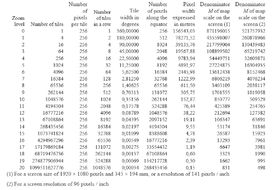
Table 1 provides basic information regarding the zoom levels of the Web Mercator projection.
The “Number of tiles” column gives the number of tiles needed to display the entire world with the given zoom level. This can be useful for calculating the amount of memory needed to store the previously generated tiles.
The "Tile width in degrees" column gives the map width in degrees of ellipsoidal length for a square tile at a specific zoom level.
The values in the column "Pixel width expressed in metres" were calculated for
a = 6378137 m, which is the major semi-axis of the ellipsoid WGS84.
The “Map scale denominator M on the screen” is calculated for the two assumed screen resolutions in which we view the map: 141 pixels / inch and 96 pixels / inch.
Table 1. Basic data on the zoom levels of the Web Mercator projection / Tablica 1. Osnovni podatci o razinama zumiranja web-Mercatorove projekcije
The proportionality factor
regulates the number of tiles, and thus the scale of the tile (scale of the part of the map) which depends on the degree or level of zoom
n. For
n = 0, a rectangular coordinate system from computer graphics was chosen, the origin of which (0,0) is in the upper left corner of the map, while the lower right corner has the coordinates (256, 256). All tiles are square in shape, but the projection is theoretically not; it is infinitely stretched in a north-south direction. Because the tiles are square in shape and have extremely large distortions in the polar regions, Google decided to show only the area that is square in the projection. It will be [-
π,
π] for the geodetic longitude
λ and [- sin
-1(tanh
π]), sin
-1 tanh
π] for the geodetic latitude
φ. In degrees it is [-180°, 180°] for geodetic longitude
λ and [-85°05112878, 85°05112878] for geodetic latitude
φ.
We are interested how the equations of the Web Mercator projection (39) written in the usual form, i.e., for the application of vector graphics, would look. We first notice the need to change the rectangular coordinate system whose origin is at the point corresponding to the ellipsoidal coordinates (
φ,
λ) = (0, 0). Furthermore, a link should be established between the raster data expressed in pixels and vector data expressed in metres. It is not difficult to see that the equator will be represented with 256 ∙ 2
n pixels, and since the equator is a circle of radius
a, its circumference in metres is 2
aπ.
Taking this into account, equations (39) pass into
These equations are simmilar to the equations of the normal aspect Mercator projection of a sphere whose radius is equal to
a (compare equations (28) and (29)). However, it is important to note that
φ and
λ in (40) are not geographical coordinates but geodetic, i.e., ellipsoidal.
At first glance, the zoom level
n is lost in (40). However, the equations of other projections are usually written for the 1:1 scale because it is assumed that they can be easily adapted to any scale 1:
M.
The resolution of the screen on which we look at the map is the ratio of the length of the screen to the number of pixels. For example, if the screen length is 345 mm and the corresponding number of pixels is 1920, the resolution
r will be 5.56 pixels per millimetre or 141 pixels per inch. This information is needed to calculate the scale of the display. Let us mark the scale of the map on the screen with 1:
M. Equalize the length of the equator
C expressed in pixels from formula (39)
C = 2x(π) = 256 ∙ 2
n
,
with the equatorial length at a scale of 1:
M expressed in pixels as a function of the resolution
r
and we will get
According to formula (43), the denominators
M of the scale represented in the last two columns inTable 1 are calculated.
It is not difficult to derive formulas for determining the distortions of the Web Mercator projection:
Formula (46) shows that the largest ratio of the linear scale factor is along the equator and that it is
It is immediately apparent that this projection is neither equidistant, nor equal-area, nor conformal. It can easily be seen that
for
φ = 0°. There is no standard parallel, i.e., a parallel along which
h =
k = 1 would be valid.
Finally, let us point out that, using the possibilities of digital technology, Google Maps shows a graphical scale on each display in the lower right corner. If we move on the map in the west-east direction or vice versa, the scale does not change because it does not depend on the geodetic longitude. If we move in a north-south direction or vice versa, the scale changes because it depends on the zoom level (Table 1).
In mid-2018, Google Maps was available online on a new mathematical basis. This is most easily seen on a map of the smallest scale. It is no longer a map of the world in the Web Mercator projection, but a map of the hemisphere in azimuthal projection (Frančula 2019).
Let us mention at the end that one can also find the unusual claim that the Web Mercator projection is neither strictly ellipsoidal nor strictly spherical (Wikipedia 2020). However, there should be no doubt because the domain of definition of that projection is the surface of a rotational ellipsoid. Therefore, it is a projection of an ellipsoid into a plane.
7. Web Mercator projection as double mapping
Stefanakis (2017) describes the origin of the Web Mercator projection in which ellipsoidal coordinates are included in the formulas of the Mercator projection for the sphere. He writes, "
Notice that the ellipsoidal coordinates of any point P were never transformed to spherical. Apparently, Google developers wanted to reduce the computational cost of transformations at the server side."Stefanakis (2017) is wrong when he says that coordinates from an ellipsoid are never transformed coordinates on a sphere. Namely, the described Google procedure by which ellipsoidal coordinates are substituted in the formulas of the normal aspect Mercator projection for mapping a sphere can be interpreted as a double projection of an ellipsoid into a plane. First the ellipsoid is mapped onto the sphere provided that the geographic coordinates on the sphere are equal to the geodetic coordinates on the ellipsoid and then the sphere is conformally mapped into the plane. To our knowledge, no one has interpreted the Web Mercator projection this way so far. InFigure 1 (Fig. 7 inStefanakis (2017) the points from the ellipsoid are mapped onto a Web Mercator projection through the opaque funnel of spherical formulas, although the figure includes the sphere.
Instead of a funnel there should have been a sphere (Fig.2).
Figure 1. Image taken fromStefanakis (2017) according to which the points from the ellipsoid are mapped through the opaque funnel. Instead of a funnel there should have been a sphere (Fig.2). / Slika 1. Slika preuzeta odStefanakisa (2017) prema kojem se točke s elipsoida kroz neprozirni lijevak sfernih formula preslikavaju u web-Mercatorovu projekciju, iako je na slici i sfera. Umjesto lijevka trebala je biti sfera (vidisl. 2).
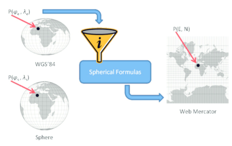
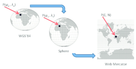
Figure 2. Image created by modification ofFigure 1. Instead of a magic funnel, a sphere was placed, thus enabling a simple explanation of the Web Mercator projection as double mapping. / Slika 2. Slika nastala modifikacijomslike 1). Umjesto čarobnoga lijevka stavljena je sfera i na taj je način omogućeno jednostavno objašnjenje web-Mercatorove projekcije kao dvostrukog preslikavanja.
Let the mapping from a rotational ellipsoid with a large semiaxis
a to a sphere of radius
R be given as follows:
R = a
φ' = φ and
λ' = λ.
In formulas (50) we denoted the geographical coordinates on the sphere with
φ
'
,
λ
'
, and the geodetic coordinates on the ellipsoid with
φ,
λ. Such a mappingKavrayskiy (1958) calls mapping in accordance with the normals (изображение с соответствием по нормалям).Hristov and Daskalova (1970) call it mapping with preserving the geographical coordinates (изображение при запазване на географските координати). The local linear scale factors of that mapping are:
The equations of the normal aspect Mercator projection are:
With the local linear scale factors
The constant K is generally determined considering that the local linear scale factor along the parallel corresponding to the latitude
φ
0
is equal to 1, hence
K = R cos φ
0
.
By definition, for the Web Mercator projection there is
φ
0
= 0 (EPSG 2014), so we have
K = R = a
So, for the Web Mercator projection, understood as double mapping we have
which are the already known formulas (42) and (43) but now derived in another way.
8. Comparison of the Mercator and the Web Mercator projection
Table 2 compares the local linear scale factors along meridians and parallels and the maximum angle distortion between the Mercator and Web Mercator projection. The Mercator projection for which the standard parallel is the equator (
K =
a) was chosen.
Table 2. Comparison of local linear scale factors along meridians and parallels and maximum angle distortion between the Mercator projection whose standard parallel is the equator and the Web Mercator projection, both for ellipsoid WGS84 / Tablica 2. Usporedba faktora lokalnih mjerila duljina uzduž meridijana i paralela i maksimalne deformacije kuta između Mercatorove projekcije kojoj je standardna paralela ekvator i web-Mercatorove projekcije, obje za elipsoid WGS84
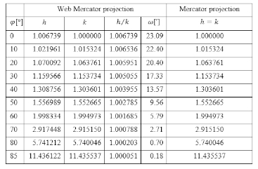
Bildirici (2015) has a similar table.Vasilca et al. (2018) investigated the differences between the Mercator and Web Mercator projections by correctly warning that they should not be equated even though they have similar names. They compared the formulas of both projections, the coordinates of a certain number of points and the borders of Romania on the maps in both projections. In conclusion, they point out: "
The Web Mercator projection features significant differences from the Mercator projection in the following aspects: the reference surface is a sphere and not an ellipsoid; …", which is not true.
9. Conclusion
In this paper, we investigated several projections of the surface of a rotational ellipsoid into a plane. We have shown that the Web Mercator projection is not a projection of a sphere onto a plane, because its domain of definition is the surface of an ellipsoid. Thus, it is one of the projections of a rotational ellipsoid in a plane although its equations are identical to the equations for the projection of a sphere. Although the equations are the same at first glance, the difference is in the area of definition of the projection. Unlike other ellipsoid projections in which the distortion distribution can be regulated by selecting the parameter we have denoted by
K in this paper, in the Web Mercator projection this is not possible, because the distortion distribution is fixed. However, this is not a disadvantage because, as with all other projections, the effect of distortion can and must be removed.
The Web Mercator projection can also be interpreted as a double mapping: mapping an ellipsoid to a sphere according to normals and then mapping a sphere to a plane according to the formulas of a Mercator projection for a sphere.
The Web Mercator projection is not a conformal projection, but it is close in properties to the Mercator projection. Naturally, the idea of web-equidistant, web-Lambert and similar projections is now emerging. These projections would be created by taking equations for mapping a sphere and substituting geodetic coordinates in them instead of geographical ones.
This way we would get approximately equidistant, approximately equal-area, etc. projections. This could be the subject of further research.
1. Uvod
Sredinom 1990-ih godina
Google je stavio na internet karte svijeta s mogućnošću zumiranja do najkrupnijih mjerila. Za izradu bilo koje karte, pa tako i spomenutih karata poznatih pod nazivom
Google Maps, potrebno je točke s plohe rotacijskog elipsoida, kojima se u geodeziji i kartografiji aproksimira nepravilna Zemljina ploha, preslikati u ravninu primjenom neke od mnogobrojnih kartografskih projekcija.
Google je u tu svrhu primijenio sljedeći postupak. U formule uspravne Mercatorove projekcije za preslikavanje sfere uvrstio je elipsoidne, tj. geodetske koordinate. Za polumjer sfere uzeta je velika poluos elipsoida WGS84 koji danas ima široku primjenu širom svijeta. Glavni razlog
Googleove primjene takvog postupka jesu jednostavnije formule za preslikavanje sfere te stoga i pet puta brže računanje nego po direktnim formulama za preslikavanje elipsoida (Zinn 2010).
Opisanim postupkom preslikavanja dobivena je nova kartografska projekcija bliska Mercatorovoj, ali bez svih svojstava Mercatorove projekcije. Stoga je ta projekcija poznata u literaturi kao web-Mercatorova projekcija, na engleskom
Web Mercator projection ili kraće
Web Mercator. Upotrebljava se i naziv
Pseudo Mercator. Web-Mercatorova projekcija je, kao i Mercatorova, uspravna cilindrična projekcija, tj. meridijani se u njoj preslikavaju kao paralelni pravci, a paralele također kao paralelni pravci okomiti na meridijane. Bitna je razlika između obje projekcije u tome što web-Mercatorova projekcija nije konformna poput Mercatorove projekcije. To znači da linearno mjerilo u web-Mercatorovoj projekciji nije u danoj točki u svim smjerovima jednako, što je svojstvo konformnih projekcija (Zinn 2010).
Opisani Googleov postupak doživio je mnogobrojne kritike. Najžešći je u kritikama bio
Geodesy Subcommittee of the Geomatics Committee of the International Association of Oil & Gas Producers - IOGP (poznat kao EPSG prema kodu koji dodjeljuje). On je odbio dati EPSG kod tom referentnom sustavu uz obrazloženje: „…
that it did not want to devalue the EPSG data collection through a system unsuited to geodesy and cartography“. Međutim, 2008. dodjeljuje mu kod EPSG:3785, ali piše: „…
that it was not an official geodetic system, since the Earth is approximated to a sphere, rather than an ellipsoid.“ Uz novi kod EPSG:3857 dodijeljen iste godine piše: „..
the WGS84 ellipsoid is applied rather than a sphere.“ U verziji 8.7 od 8. rujna 2014. dan je komentar: „
Uses spherical development of ellipsoidal coordinates. Relative to WGS 84 / World Mercator (CRS code 3395) errors of 0.7 percent in scale and differences in northing of up to 43 km in the map (equivalent to 21 km on the ground) may arise” (EPSG 2014). U navedenoj se rečenici spominje riječ errors (pogreške), što nije u skladu s teorijom kartografskih projekcija jer je riječ o deformacijama, a ne pogreškama.
Iz navedenih je citata vidljivo koliko je vremena trebalo da EPSG utvrdi da se u web-Mercatorovoj projekciji ne radi o preslikavanju sfere, nego elipsoida i da je 43 km u razmaku između paralela razlika između Mercatorove i web-Mercatorove, a ne pogreška web-Mercatorove projekcije. Zbog ugleda koji EPSG u svijetu uživa, mnogi su citirali njihove izjave smatrajućih ih neprikosnovenima (Favretto 2014).
Nedostatak web-Mercatorove projekcije dolazi do izražaja praktički jedino u najsitnijim mjerilima kada je cijeli svijet, ili najveći njegov dio, vidljiv na ekranu. Tada smetaju velike deformacije površina, posebno u sjevernim dijelovima Zemljine sfere. Kartografi često navode kao primjer Grenland koji je na karti gotovo jednako velik kao Afrika iako je od nje oko 14 puta manji. Stoga su kartografi posljednjih desetljeća često upozoravali da Mercatorova projekcija, ali i ostale uspravne cilindrične projekcije, nisu prikladne za izradu općegeografskih karata svijeta (Committee on Map Projections 1989).
Pretpostavljamo da je zbog svih tih kritika
Google sredinom 2018. izradio i novu matematičku osnovu
Google Mapsa (u izborniku treba kliknuti
Globe). Najlakše je to zamjetljivo na karti najsitnijeg mjerila. To više nije karta svijeta u web-Mercatorovoj projekciji, već karta hemisfere u azimutnoj projekciji. Međutim, karte srednjih i krupnih mjerila, kojima se korisnici najviše služe u određivanju rute između dviju točaka, i dalje su u web-Mercatorovoj projekciji (Frančula 2019).
Sadržaj ovog članka organiziran je tako da se u drugom poglavlju podsjeća na geodetsku parametrizaciju rotacijskog elipsoida, a u trećem, vrlo kratko, na projekcije plohe elipsoida u ravninu. Četvrto je poglavlje posvećeno cilindričnim projekcijama elipsoida jer web-Mercatorova projekcija pripada toj skupini projekcija. U petom se poglavlju daju primjeri ekvidistantne, ekvivalentne, konformne i perspektivne projekcije elipsoida kako bi se na prirodan način moglo zaključiti da i web-Mercatorova projekcija, o kojoj je riječ u šestom poglavlju, pripada istoj skupini projekcija. U sedmom poglavlju pokazujemo da se web-Mercatorova projekcija može interpretirati i kao dvostruko preslikavanje koje se sastoji od preslikavanja elipsoida na sferu i zatim sfere u ravninu. U osmom poglavlju dajemo usporedbu Mercatorove i web-Mercatorove projekcije, a u devetom donosimo zaključke o provedenim istraživanjima.
2. Geodetska parametrizacija rotacijskog elipsoida
Rotacijski elipsoid s poluosima
a i
b i sa središtem u ishodištu pravokutnog koordinatnog sustava u prostoru ima jednadžbu
Ta se ploha može doživjeti i kao slika preslikavanja opisanog formulama
gdje su
Preslikavanje (2)-(4) naziva se geodetska parametrizacija rotacijskog elipsoida (1), a omogućava nam da točke s koordinatama (
X,
Y,
Z) na plohi elipsoida identificiramo s točkama kojima odgovaraju geodetske koordinate (
φ,
λ).
Nije teško dobiti prvu diferencijalnu formu preslikavanja (2)
gdje je
3. Projekcije elipsoida u ravninu
MKartografska se projekcija obično definira kao preslikavanje plohe elipsoida u ravninu s pomoću formula
x = x(φ, λ),
y = y(φ, λ),
gdje su
x i
y koordinate u pravokutnom (matematičkom, desno orijentiranom) koordinatnom sustavu u ravnini, a
λ ∈ [-
π,
π],
geodetske koordinate, širina i dužina. Pri tome smo u mislima identificirali točke na elipsoidu (1) s njihovim geodetskim koordinatama (4) na temelju veze (2). Jasno je da, teorijski gledano, ima beskonačno mnogo preslikavanja (7) iako ona ne mogu biti baš bilo kakva da bi rezultat bio onakav kakav ga obično doživljavamo. Obično se pretpostavlja da su funkcije u izrazu (7) po dijelovima neprekidne i derivabilne.
Prva diferencijalna forma preslikavanja (7) je
ds'
2 = Edφ
2 + 2Fdφdλ + Gdλ
2
,
gdje su koeficijenti
Faktor lokalnog linearnog mjerila
c za preslikavanje (7) definira se u teoriji kartografskih projekcija relacijom
a važan je pri određivanju distorzija ili deformacija nastalih zbog projekcije.
4. Cilindrične projekcije
Neke su od kartografskih projekcija cilindrične i u ovom ćemo se članku baviti samo takvima. Cilindrične projekcije u uspravnom aspektu ili uspravne cilindrične projekcije su takve projekcije kod kojih su slike paralela normalne mreže međusobno paralelne dužine, a slike meridijana pravci okomiti na slike paralela (Tobler 1962). Cilindrične projekcije, kod kojih su slike meridijana udaljene od slike srednjeg meridijana područja preslikavanja proporcionalno razlici njihovih geografskih dužina, zvat ćemo konvencionalnim cilindričnim projekcijama. Za konvencionalne cilindrične projekcije jednadžbe glase
x = K(λ - λ
0)
,
y = y(φ),
gdje je
K>0 konstanta proporcionalnosti, a
λ
0
geodetska dužina odabranog srednjeg meridijana,
λ ∈ [-π, π]
,
a funkcije u (11) su neprekidne i monotono rastuće. Pri tome su, kao i kod svake kartografske projekcije,
x i
y koordinate točke u pravokutnom (matematičkom, desnom) koordinatnom sustavu u ravnini. Kao što se lijepo vidi, riječ je o preslikavanju u ravninu, a ne na plašt cilindra.
Za cilindrične projekcije (11) imamo prema (9)
pa je prva diferencijalna forma tog preslikavanja prema (8), (9) i (12)
Kvadrat faktora lokalnog mjerila duljina
c za cilindrične projekcije elipsoida u ravninu (11) je dakle
Iz (14) se lako dobije faktor lokalnog mjerila duljina u smjeru meridijana (
dλ = 0)
i faktor lokalnog mjerila duljina u smjeru paralela meridijana (
dφ = 0)
Za
k = 1 geodetska širina
φ iz (16) odgovarat će ekvidistantnoj paraleli. Ako je to ekvator, onda je
K =
a.
Faktor lokalnog mjerila površina bit će
Za maksimalnu deformaciju kuta
ω vrijedi poznata formula
ω
5. Primjeri cilindričnih projekcija elipsoida
5.1. Ekvidistantna cilindrična projekcija elipsoida
Jednadžbama
definirana je ekvidistantna cilindrična projekcija elipsoida, ako su
φ i
λ geodetska širina, odnosno dužina,
K,
φ
0
i
λ
0
konstante, a
M polumjer zakrivljenosti meridijana definiran relacijom (6). Integral u (19) predstavlja duljinu luka meridijana. To je eliptički integral koji nije moguće izraziti s pomoću elementarnih funkcija. Geodetska širina
φ
0
može se izabrati po volji. Uz izbor
φ
0
= 0 ekvator će se preslikati na koordinatnu os
x. Ako je
K =
a, duljina slika svih paralela bit će 2
aπ.
Lako se vidi da iz (19) slijedi
tj. stvarno je riječ o ekvidistantnoj projekciji uzduž meridijana. Za tu je projekciju
5.2. Ekvivalentna ili Lambertova cilindrična projekcija elipsoida
Jednadžbama
definirana je ekvivalentna cilindrična projekcija elipsoida, gdje su
φ i
λ geodetska širina, odnosno dužina,
K,
φ
0
i
λ
0
konstante,
M polumjer zakrivljenosti meridijana definiran relacijom (6), a
N polumjer zakrivljenosti presjeka po prvom vertikalu definiran relacijom (3). Integral u (23) predstavlja površinu elipsoidnog trapeza kojemu su stranice ∆
λ = 1 i ∆
φ =
φ -
φ
0
. Taj se integral može izraziti s pomoću elementarnih funkcija pa umjesto (23) možemo napisati
Konstanta
φ
0
može se izabrati po volji. Uz izbor
φ
0
= 0 ekvator će se preslikati na koordinatnu os
x.
Na temelju (24) možemo izračunati
pa je onda
p = hk = 1,
tj. stvarno je riječ o ekvivalentnoj projekciji. Za tu je projekciju
5.3. Konformna ili Mercatorova cilindrična projekcija elipsoida
Jednadžbama
definirana je konformna cilindrična projekcija elipsoida, gdje su
φ i
λ geodetska širina, odnosno dužina,
K,
φ
0
i
λ
0
konstante,
M polumjer zakrivljenosti meridijana definiran relacijom (6), a
N polumjer zakrivljenosti presjeka po prvom vertikalu definiran relacijom (3). Konstanta
φ
0
može se izabrati po volji. Uz izbor
φ
0
= 0 ekvator će se preslikati na koordinatnu os
x. Integral u (28) je integral izometrijske širine koji se može izraziti s pomoću elementarnih funkcija na više načina:
Lako se vidi da vrijedi
tj. da je stvarno riječ o konformnoj projekciji. Za tu je projekciju
Za
K =
a uzduž ekvatora bit će
h =
k = 1, tj. ekvator će biti standardna paralela. Za
K =
N(
φ
1
)
cos
φ
1
standardna paralela bit će ona paralela kojoj odgovara geodetska širina
φ
1
. Prema tome, promjena konstante
K je s jedne strane promjena standardne paralele, a istodobno i promjena mjerila karte.
Mnogi autori definiraju Mercatorovu projekciju elipsoida stavljajući
K =
a (Thomas 1952,Snyder 1987,Osborne 2013 i drugi). Međutim, to ne mora uvijek biti tako. Podsjetimo se tzv.
konstrukcijske širine (geodetska širina standardne paralele, eng.
mean latitude) koja se upotrebljava pri izradi pomorskih navigacijskih karata (Kavrayskiy 1959,Peterca i dr. 1974,Vahrameyeva i dr. 1986,Bugayevskiy 1998). To je geodetska širina one paralele koja prolazi središnjim dijelom pomorske karte i koja je standardna paralela za taj list karte. Na temelju te širine određuje se konstanta
K u jednadžbama Mercatorove projekcije i na taj se način utječe na razdiobu distorzija na karti.
5.4. Perspektivna projekcija elipsoida na plašt valjka
Jednadžbama
x = K(λ - λ
0)
,
y = K(1 - e
2) tan φ
.
definirana je perspektivna projekcija elipsoida iz njegova središta na plašt kružnog valjka kojem se os poklapa s koordinatnom osi
Z, a polumjer mu je
K. Pri tome su
φ i
λ geodetska širina, odnosno dužina,
λ
0
konstanta.
Lako se vidi da vrijedi
Odmah se vidi da ta projekcija nije ni ekvidistantna, ni ekvivalentna, ni konformna. Ako je
K =
a, onda je ekvator standardna paralela, tj. onda za točke na ekvatoru vrijedi
h =
k = 1.
6. Web-Mercatorova projekcija elipsoida
Jednadžbama
definirana je web-Mercatorova projekcija elipsoida prilagođena rasterskim podatcima, gdje su
φ i
λ elipsoidna širina i duljina, a
n razina zumiranja (Wikipedia 2020).
Utablici 1 dani su osnovni podatci u vezi s razinama zumiranja web-Mercatorove projekcije.
Stupac "Broj pločica" daje broj pločica potreban za prikaz cijelog svijeta uz zadanu razinu zumiranja. To može biti korisno za računanje količine memorije potrebne za čuvanje prethodno generiranih pločica.
Stupac "Širina pločice u stupnjevima" daje širinu karte u stupnjevima elipsoidne dužine za kvadratnu pločicu na određenoj razini zumiranja.
Vrijednosti u stupcu " Širina piksela izražena u metrima" izračunane su za
a = 6378137 m, što je velika poluos elipsoida WGS84.
" Nazivnik mjerila
M karte na zaslonu" izračunan je za dvije pretpostavljene rezolucije zaslona na kojem gledamo kartu: 141 piksel/inču i 96 piksela/inču.
Faktorom proporcionalnosti
regulira se broj pločica (
tiles), a time i mjerilo pločice (mjerilo dijela karte) koje ovisi o stupnju ili razini zumiranja
n.
Za
n = 0 odabran je pravokutni koordinatni sustav iz računalne grafike kojem je ishodište (0,0) u gornjem lijevom kutu karte, a donji desni kut ima koordinate (256, 256).
Sve su pločice kvadratnog oblika, no projekcija teorijski nije, nego je beskonačno rastegnuta u smjeru sjever-jug. Budući da su pločice kvadratnog oblika i da su u polarnim područjima izrazito velike distorzije, Google je odlučio prikazati samo područje koje u projekciji čini kvadrat. To će biti [-
π,
π] za geodetsku dužinu
λ i [- sin
-1(tanh
π]), sin
-1tanh
π] za geodetsku širinu
φ. U stupnjevima to je [-180°, 180°] za geodetsku dužinu
λ i [-85°05112878, 85°05112878] za geodetsku širinu
φ.
Zanima nas kako bi izgledale jednadžbe web-Mercatorove projekcije (39) zapisane u uobičajenom obliku, odnosno za primjenu vektorske grafike. Najprije uočimo potrebu promjene pravokutnog koordinatnog sustava kojem je ishodište u točki koja odgovara elipsoidnim koordinatama (
φ,
λ) = (0, 0). Nadalje, treba uspostaviti vezu između rasterskih podataka izraženih u pikselima i vektorskih izraženih u metrima. Nije teško vidjeti da će ekvator biti prikazan s 256 ∙ 2
n piksela, a budući da je ekvator kružnica polumjera
a, njegov opseg u metrima je 2
aπ. Uzevši u obzir navedeno, jednadžbe (39) prelaze u
Te su jednadžbe nalik na jednadžbe uspravne Mercatorove projekcije sfere kojoj je radijus jednak
a (usporediti jednadžbe (28) i (29)). No važno je uočiti da
φ i
λ u (40) nisu geografske koordinate, nego geodetske, tj. elipsoidne.
U tim se jednadžbama na prvi pogled izgubila razina zumiranja
n. Međutim, i jednadžbe drugih projekcija obično pišemo za mjerilo 1 : 1 jer se podrazumijeva da se one lako mogu prilagoditi bilo kojem mjerilu 1 :
M.
Rezolucija zaslona na kojem gledamo kartu omjer je duljine zaslona i broja piksela. Tako npr. ako je duljina zaslona 345 mm, a odgovarajući broj piksela 1920, rezolucija
r će biti 5,56 piksela po milimetru ili 141 piksel po inču. Taj je podatak potreban da bi se izračunalo mjerilo prikaza na zaslonu. Označimo mjerilo prikaza karte na zaslonu s 1 :
M. Izjednačimo duljinu ekvatora
C izraženu u pikselima iz formule (39)
C = 2x(π) = 256 ∙ 2
n
,
s duljinom ekvatora u mjerilu 1 :
M izraženom u pikselima u ovisnosti o rezoluciji
r
i dobit ćemo
Po formuli (43) izračunani su nazivnici mjerila
M u posljednja dva stupca utablici 1.
Nije teško izvesti formule za određivanje distorzija web-Mercatorove projekcije:
Formula (46) pokazuje da je najveći omjer faktora mjerila duljina uzduž ekvatora i da iznosi
Odmah se vidi da ta projekcija nije ni ekvidistantna, ni ekvivalentna, ni konformna. Lako se može vidjeti da je
za
φ = 0°. Standardna paralela, tj. paralela uzduž koje bi vrijedilo
h =
k = 1, ne postoji.
Na kraju istaknimo da, služeći se mogućnostima digitalne tehnologije,
Google Maps na svakom prikazu u donjem desnom uglu prikazuje grafičko mjerilo. Pomičemo li se po karti u smjeru zapad-istok ili obrnuto, mjerilo se ne mijenja jer ono ne ovisi o geodetskoj dužini. Pomičemo li se u smjeru sjever-jug ili obratno, mjerilo se mijenja jer ovisi o razini zumiranja (tablicA 1).
Sredinom 2018.
Google Maps je bio dostupan na internetu u novoj matematičkoj osnovi. Najlakše je to zamjetljivo na karti najsitnijeg mjerila. To više nije karta svijeta u web-Mercatorovoj projekciji, već karta polusfere u azimutnoj projekciji (Frančula 2019).
Spomenimo na kraju da se može naći i neobična tvrdnja da web-Mercatorova projekcija nije ni elipsoidna ni sferna: "
The projection is neither strictly ellipsoidal nor strictly spherical." (Wikipedia 2020). Međutim, dvojbe ne bi trebalo biti jer je područje definicije ili domena te projekcije ploha rotacijskog elipsoida. Prema tome, riječ je o projekciji elipsoida u ravninu.
7. Web-Mercatorova projekcija kao dvostruko preslikavanje
Stefanakis (2017) opisuje nastanak web-Mercatorove projekcije u kojoj su u formule Mercatorove projekcije za sferu uvrštene elipsoidne koordinate. Pri tome piše: „
Notice that the ellipsoidal coordinates of any point P were never transformed to spherical. Apparently, Google developers wanted to reduce the computational cost of transformations at the server side.“Stefanakis (2017) nije u pravu kad kaže da koordinate s elipsoida nisu nikad transformirane koordinate na sferi. Naime, opisani
Googleov postupak, kojim je u formule uspravne Mercatorove projekcije za preslikavanje sfere uvrstio elipsoidne koordinate, može se interpretirati kao dvostruka projekcija elipsoida u ravninu. Prvo je elipsoid preslikan na sferu uz uvjet da su koordinate na sferi jednake koordinatama na elipsoidu i potom je sfera konformno preslikana u ravninu. Prema našem saznanju nitko do sada nije interpretirao web-Mercatorovu projekciju na taj način. NaSLICI 1 (sl. 7 kodStefanakisa (2017)) točke s elipsoida kroz neprozirni lijevak sfernih formula preslikavaju se u web-Mercatorovu projekciju, iako je na slici i sfera. Umjesto lijevka trebala je biti sfera (sl.2).
Neka je preslikavanje s rotacijskog elipsoida s velikom poluosi
a na sferu polumjera
R zadano ovako:
R = a
φ' = φ i
λ' = λ.
U formulama (50) označili smo geografske koordinate na sferi s
φ
'
,
λ
'
, a geodetske koordinate na elipsoidu s
φ,
λ. Takvo preslikavanjeKavrayskiy (1958) naziva preslikavanje u skladu s normalama (изображение с соответствием по нормалям).Hristov i Daskalova (1970) nazivaju ga preslikavanje koje čuva geografske koordinate (изображение при запазване на географските координати).Faktori lokalnog mjerila duljina za to preslikavanje su:
Jednadžbe uspravne Mercatorove projekcije sfere su:
s faktorom lokalnog mjerila duljina
Konstanta K je općenito određena uz uvjet da faktor lokalnog mjerila duljina uzduž paralele kojoj odgovara širina
φ
0
bude jednak 1, odakle slijedi da je
K = R cos φ
0
.
Po definiciji za web-Mercatorovu projekciju vrijedi
φ
0
= 0 (EPSG 2014), pa imamo
K = R = a
Dakle, za web-Mercatorovu projekciju, shvaćenu kao dvostruko preslikavanje, imamo
što su već poznate formule (42) i (43) izvedene na drugi način.
8. Usporedba Mercatorove i web-Mercatorove projekcije
Utablici 2 dajemo usporedbu faktora lokalnih mjerila duljina uzduž meridijana i paralela i maksimalne deformacije kuta između Mercatorove i web-Mercatorove projekcije. Pri tom je odabrana Mercatorova projekcija za koju je standardna paralela ekvator (
K =
a).
Sličnu tablicu imaBildirici (2015).Vasilca i dr. (2018) istražili su razlike između Mercatorove i web-Mercatorove projekcije pravilno upozoravajući da ih se, iako imaju slična imena, ne smije poistovjetiti. Usporedili su formule jedne i druge projekcije, koordinate određenog broja točaka i granice Rumunjske na kartama u obje projekcije. U zaključku ističu: ”
Web Mercator projection features significant differences from the Mercator projection in the following aspects: the reference surface is a sphere and not an ellipsoid;…“, što nije točno. Referentna ploha u obje projekcije je elipsoid WGS 84.
9. Zaključak
U ovome smo radu istražili nekoliko projekcija plohe rotacijskog elipsoida u ravninu. Pokazali smo da web-Mercatorova projekcija nije projekcija sfere u ravninu jer je njezino područje definicije, odnosno domena, ploha elipsoida. Dakle, to je jedna od projekcija rotacijskog elipsoida u ravninu premda su njezine jednadžbe istovjetne jednadžbama za projekciju sfere. Iako su jednadžbe na prvi pogled iste, razlika je u području definicije projekcije. Za razliku od ostalih projekcija elipsoida kod kojih se razdioba deformacija može regulirati izborom parametra koji smo u ovom članku označili s
K, kod web-Mercatorove projekcije to nije moguće. Kod nje je razdioba deformacija fiksirana. Međutim, to nije nedostatak jer se, kao i kod svih drugih projekcija, utjecaj deformacija može i mora ukloniti.
Web-Mercatorova projekcija može se interpretirati i kao dvostruko preslikavanje: preslikavanje elipsoida na sferu po normalama i preslikavanje sfere u ravninu po formulama Mercatorove projekcije za sferu.
Web-Mercatorova projekcija nije konformna projekcija, ali je po svojstvima bliska Mercatorovoj projekciji. Prirodno se sad pojavljuje ideja o web-ekvidistantnoj, web-Lambertovoj i sličnim projekcijama koje nastaju tako da se uzmu jednadžbe za preslikavanje sfere i u njih, umjesto geografskih, uvrste geodetske koordinate. Na taj bismo način dobili približno ekvidistante, približno ekvivalentne itd. projekcije. Možda bi to mogla biti tema daljnjih istraživanja.
