
1. INTRODUCTION
Problems connected with lateral vibrations of beams have received a lot of attention in scientific literature over the past several decades because they translate well into a wide range of engineering problems in which distributed elasticity plays a dominant role in the response of structures deflected from their equilibrium and/or subjected to dynamic loads. Depending on the level of complexity of the studied problem, the task of finding the natural frequencies and mode shapes often involves a dose of cumbersome mathematics if the solutions are to be sought in closed form. The necessity to resort to advanced mathematical concepts (e.g. Green’s functions) on one hand is on the other counterbalanced by the ever-increasing CPU computing power and the rapid development of CAD and FEM software solutions. The problem was also tackled by resorting to approximate solutions, either in the form of rule-of-thumb formulas intended for the preliminary engineering estimation of natural frequencies, or in the form of more elaborate analytic approach of series solutions and numerical formulations that lead to systems of linear algebraic equations, both of which are capable of producing mode shapes as well.
The problem of free transverse vibrations of beams, which is of central interest in this paper, has been studied extensively, to varying degrees of complexity and with various types of boundary conditions and intermediate restraints. This field of study can generally be divided into several classes of problems, such as, for instance, the problem of elastically supported beam (Kukla, 1991) , the problem of a beam with lumped masses (Skoblar et al., 2017) , the problem of a beam with elastically mounted masses (Kukla, Posiadala, 1994) , the problem of a beam with moving masses, as well as a combination of some of the previous cases (Mohamad, 2003) . The problem of elastic support of beams, which is considered in this paper, is, for instance, encountered in problems involving vibrations of railway tracks (Connolly et al., 2014) , the propagation of sound through periodically supported panels etc. (Mead, Pujara, 1971, Legault, Mejdi, Atalla, 2011) .
Free vibration of an Euler-Bernoulli beam with translational and torsional linear springs was studied by (Bergman, McFarland, 1988) by using the Green’s functions. The Green’s function method was also utilized to study the free transverse vibrations of Euler-Bernoulli beams with intermediate elastic supports (Kukla, 1991) and with many elastically mounted masses (Kukla, Posiadala, 1994) . The closed form expressions of the equations for the natural frequencies were obtained. In paper (Kukla, 1997) the Green’s function method was applied to calculate the natural frequencies of a Timoshenko beam with multi-mass oscillators. Tables of Green’s functions for the theory of beam vibrations with general intermediate appendages can be found in (Mohamad, 1994) . In (Abu-Hilal, 2003) the Green’s function method is used for determining the dynamic response of Euler-Bernoulli beams subjected to distributed and concentrated loads. Also, the Green’s functions for various beams with different homogenous and elastic boundary conditions are given. Free vibration analysis was studied by (Skoblar et al., 2017) , who derived the characteristic equation for a cantilever Euler-Bernoulli beam carrying a point mass by Laplace transform method. The characteristic equation was solved and exact natural frequencies and normal modes were obtained.
In this paper the problem of an Euler-Bernoulli beam elastically supported with translational springs is examined and the results obtained with three different approaches are compared.
The main comparison is made between two analytic methods, namely the method of Laplace transforms and the method of Green’s functions. These two methods are complemented with numerical results obtained by FEM, which are also used to verify the analytic results. Chapter 2 gives a theoretical foundation for the implementation of the Laplace transform method and the Green’s function method. Theoretical considerations are further elaborated with an example solved in Chapter 3, and the results are compared to the results obtained by FEM in Femap v10. Chapter 4 discusses various aspects of the three employed approaches in free vibration analysis of beams, with an emphasis on their respective advantages and disadvantages. Finally, concluding remarks are given in Chapter 5.
2. FORMULATION OF THE PROBLEM
2. 1 General considerations
A beam supported elastically by a number of translational springs is shown in Figure 1, with a set of boundary conditions (B.C.) defined at x = 0 and x = L . For the sake of generality no assumptions are made beforehand as to the number and exact positions of the springs, and the governing equations and the resulting solutions are given in generalized form.
The transverse displacement w(x,t) of a freely vibrating beam supported by translational springs as shown in Figure 1 is generally governed by the equation:
where w(x,t) is the beam deflection at cross-section x at time t, E is the modulus of elasticity, I is the beam cross-sectional moment of inertia, ρ is the density, A is the cross-sectional area of the beam, and k(x) is the stiffness of the foundation of the beam at position x .
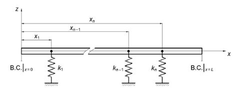
When the beam is supported by N linear springs at points xn, with n = 1, N, it can be stated that
where kn is the stiffness of the n-th translational spring (located at xn), and d is the Dirac delta function with the properties:
The solution for the transverse displacement of any point along the beam in time is assumed as the product of two functions. One function is dependent only on the spatial coordinate x, and thus qualitatively describes the deflected form of the vibrating beam, i.e. its mode shape. The second function is a harmonic function dependent only on time t, which thus scales the first function (i.e. the deflections) as the progression of time varies its value. We, therefore, assume the solution of Eq. (1) in the following form:
where ω is the natural frequency of the beam. Using Eq. (4), from (1) it is easy to obtain:
After substituting expressions (2) and (5) into (1), Eq. (1) can be rewritten as:
By introducing the non-dimensional variables:
where L is the length of the beam, from (6) it can finally be derived that
where and . We shall hereafter refer to ε as the frequency coefficient and to Kn as the non-dimensional stiffness.
The differential equation in (8) is solved in this paper using the Laplace transform and the Green’s function approach.
2. 2 Laplace transform method
Applying the Laplace transform to Eq. (8) and knowing that
where L is the Laplace operator, the Laplace transformed solution with respect to the non-dimensional position variable ξ is obtained as
Finally, assuming the pinned-pinned boundary conditions:
and taking the first two, equation (10) yields
The inverse transform of (12) is found to be
(13)
where H(·) is the Heaviside function. Using the last two boundary conditions in (11), the two unknown constants )0(~W′ and )0(~W′′′ in (13) are obtained, yielding finally the mode shape function:
(14)
To the best of the authors’ knowledge, the generalized mode shape equation (14) for pinned-pinned beam supported with an arbitrary number of translational springs of varying stiffness has not been presented in such a form in existing literature.
If there is only one spring, applied at ξ=ξ1, equation (14) can easily be transformed into the frequency equation, whose solutions are the values of the frequency coefficient ε:
This procedure can be repeated for any number of springs ξm (m = 1,...,N), in which case Eq. (14) is most suitably written in matrix form. For reasons of simplicity and to avoid repetition, this principle is demonstrated in section 2.3.1.
2. 3 Green’s function method
2.3.1 General considerations
By using the standard property of the Dirac delta function in (3.a), Eq. (8) is transformed into:
Furthermore, if G(x,x<sub>n</sub>) is the Green’s function of the stated problem, which by definition is the solution of a differential equation when the forcing term equals the Dirac delta function,
then using the property in (3.b) yields the solution of Eq. (16) as
Allowing ξ in Eq. (18) to assume values ξm (m = 1,...,N) forms a system of N linear equations
which can be represented in matrix form as
where
(21)
Each m-th equation in this system of equations can be understood as the calculation of the non-dimensional deflection )(~mWx at point ξm. The quantity ),(nmGxx determines the influence spring kn exerts at point ξm – that is, ),(nmGxx multiplied by Kn yields the amount contributed by spring kn (which is applied at point ξn) to the overall non-dimensional deflection at point ξm.In order to determine the eigenvalues of the system, the determinant of the matrix K must be set equal to zero:
which constitutes the frequency equation of the system, whose solutions are the values of the frequency coefficient ε. Finally, the natural frequencies are obtained as:
For each value of ε, the corresponding mode shape can be determined from expression (18) as:
where represents the modal deflection, as the deflection relative to the non-dimensional deflection at the point of application of the first spring.
2.3.2 Determination of the Green’s function
The Green’s function to be used in the procedure described above can be determined from Eq. (17), by applying any method conventionally used for solving differential equations. For instance, equation (17) could be solved very effectively by means of Laplace transforms, or using the method of parameter variation. For the purpose of this investigation, the method of undetermined coefficients is employed. It is obvious that for ξ=ξn Eq. (17) is homogeneous, i.e. the right hand side is equal to zero. In such a case it can be shown that the solution consists of linear superpositions of sin(εξ), cos(εξ), sinh(εξ) and cosh(εξ) on either side of ξ=ξn and can generally be assumed in the following form:
In order to determine the eight constants (C1...C8), the function G(ξ,ξn) must first satisfy four boundary conditions, two at each end of the beam (ξ=0 and ξ= 1), which depend on the type of the end support. For the case of a pinned-pinned beam these conditions are:
Since the problem is governed by a fourth-order differential equation (r= 4), the remaining four constraints necessary for the calculation of all constants follow from the fact that G(ξ,ξn) and its derivatives up to the order of two (r– 2) satisfy the continuity conditions at point ξ=ξn, and the (r– 1)th derivative has a discontinuity of 1/an(ξn) at the same point; here, an is the coefficient multiplying the highest derivative in (17), in this case an= 1 (Riley et al., 2006) :
Using conditions given in Eqs. (26) and (27) the coefficients C5...C8 can be expressed in terms of C1...C4 as:
where . These generally valid expressions can now be used with exact boundary conditions (26) to determine the Green’s function formulated in Eq. (25). Finally, the Green’s function for the pinned-pinned boundary conditions is obtained as:
where
Once that the Green’s function is derived, the mode shape equation (18) can be transformed into (14), which is obtained by the Laplace transform method.
3. EXAMPLE
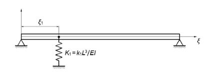
If a beam is supported with only one spring the frequency equation in (22) reduces to:
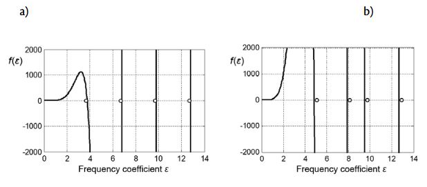
Assuming the beam is pinned at both ends (Figure 2), we can use expressions (29) and (30) for the calculation of the natural frequencies and mode shapes. After minor manipulations, Eq. (31) can be shown to be mathematically equivalent to the frequency equation (15) obtained by the Laplace transform method. As already pointed out in preceding sections, the natural frequencies can be calculated from the frequency coefficients, obtained in this case as the roots of Eq. (31). This is shown in the two diagrams in Figure 3 for two different positions ξ1 of the spring; an i-th zero of each curve (counted from the left) is equal to the value of the frequency coefficient εi corresponding to the i-th natural frequency.
Source: Authors’ original work
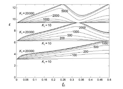
Plotting the frequency coefficients against all possible positions ξ1 of the spring for a chosen set of different values of the non-dimensional stiffness produces the diagram shown in Figure 4. Here, each plotted curve shows the change of the natural frequency with respect to the position of the spring for a constant value of K1
Additional insight into these results can be obtained by plotting the frequency coefficients as functions of the non-dimensional stiffness while the position of the spring is held constant, as shown in Figure 5.
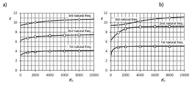
Source: Authors’ original work
Considering that the Green’s function for this problem is defined with Eq. (29), the expression for mode shapes (24) can be rewritten as:
where the properties of the Heaviside function prove convenient in the implementation of an automated computer code.
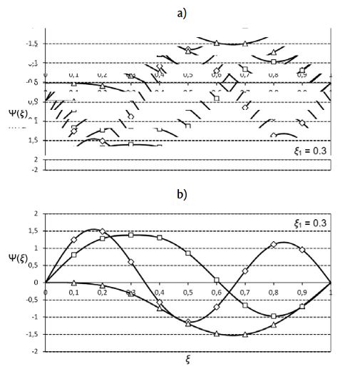
Comparison of the mass-normalized mode shapes, as described in more detail in (Skoblar et al., 2017) , is shown in Figure 6.
4. DISCUSSION
It has already been pointed out that the frequency equations derived by the Laplace method and the Green’s function method are mathematically equivalent, and therefore both methods yield accurate solutions in closed form. The mode shape equation from (14), determined with Laplace transforms, incorporates the Heaviside function, but it can easily be transformed into a more familiar form (18), which is obtained as an intermediate step in the derivation of the Green’s function.
Although the Laplace method is easier to use and implement from the standpoint of mathematical structure, the two analysed methods can be equally appropriate in free vibration analysis, i.e. for the calculation of natural frequencies and natural modes. However, the advantage of the Green’s function method lies in the fact that for different boundary conditions Green’s functions are already known from the available publications (Mohamad, 1994, Abu-Hilal, 2003) and, therefore, the calculation of eigenmodes (18) can be carried out more easily than by directly applying the Laplace transform method. Furthermore, the Green’s function method lends itself easily to the analysis of forced vibrations. The method of Green’s functions is also more efficient than the series methods, because it yields exact solutions in closed form, which is particularly important in the determination of dynamic responses of beams. It must be noted that the boundary conditions are embedded in the Green’s functions, and therefore it is not necessary to determine the eigenvalues and the corresponding eigenfunctions in order to determine the dynamic responses, which is required with series solutions (Abu-Hilal, 2003) .
Free vibration analysis with FEM is not computationally demanding by present-day standards, and it takes only seconds for the solution to converge. As shown in Figures 5 and 6, the results conform almost perfectly to the analytical solutions for both the natural frequencies and mode shapes. In fact, since the difference of natural frequencies is of the order of 10–4, these can be considered as accurate results by any engineering standard. This is especially significant in engineering practice, since able use of FEM software packages does not require any kind of theoretical insight and understanding of the underlying mathematics on part of the designer. However, there are two principal disadvantages of the FEM analysis. Firstly, the user is faced with the requirement for pre-processing whenever a single parameter in the model is changed (e.g. spring stiffness and/or spring position), which can often be more time consuming than the analysis itself. Secondly, the inability to produce generalized results mandates additional calculations and manipulations with the simulation output data in the interpretation and post-processing phase in order to transform the obtained results from a case-specific form into a universally valid form.
5. CONCLUSION
In this paper a comparison between two analytic methods for the determination of natural frequencies and mode shapes of Euler-Bernoulli beam supported by an arbitrary number of translational springs of varying stiffness is presented. The problem of free vibrations is solved with the method of Laplace transforms and with the Green’s function method. Although, from the standpoint of mathematical structure, the Laplace transform method seems to be easier to use and implement, the resulting formulas of the two methods are found to be algebraically equivalent. Finally, analytical solutions are compared to the results obtained by FEM analysis for the case when the beam is supported with a single spring. Excellent agreement between the analytical solutions and numerical results is achieved, which shows that the two methods are equally appropriate for the calculation of natural frequencies and natural modes.
Moreover, the generalized mode shape equation obtained with the Laplace transform method can be used very effectively for the calculation of natural modes of an arbitrary beam with an arbitrary number of springs for the case of pinned-pinned boundary conditions.