
INTRODUCTION
Globalization, internationalization, and privatization have all done much to shape the current situation of higher education in Europe, as well as in Bosnia and Herzegovina. Namely, state control is giving way to more institutional management in the name of efficiency and responsiveness to society’s diverse needs, proven through new processes of accountability and quality assurance. One of the results is the adoption of more market-type mechanisms and modern types of governance[1]. Today’s higher education institutions (HEIs) are under a considerable challenge to prepare students for entry into a highly competitive, globalized, dynamic, high-tech, complex and interdisciplinary business environment. HEIs can respond to that challenge by equipping their students with appropriate skills, knowledge, values, and attributes. There is a strong drive to build and create knowledge together with an understanding of working life and reformulate the concept of knowledge in education institutions[2]. Transformations are experienced by all stakeholders in the educational process: governments’ bodies, HEIs management, teachers, students, and administration. Although most universities have developed teaching and learning strategies, they still struggle to implement them and effectively assess their impact on the learning experience. It is hard to find a way to match the overall learning needs of students with curriculum development and to ensure programs are relevant for students living in a globalized world[3]. One of the significant changes in the education market is the emerging of corporate education as a form of informal learning. Companies, through specialist courses, educate their staff (and others on the labor market) according to their current needs. Although this type of education cannot be compared with formal education, it is a fact and, as such, must be considered[4]. Corporate education is focused on modules and flexible and personalized knowledge delivery; as such, it could indicate a direction that might prove unavoidable by formal education institutions. For example, a corporation offers a comprehensive list of short-term specialized courses to its employees, helping a learner navigate through learning paths[5][6]. Such learning delivery platforms put pressure on institutions offering formal education to upgrade their curriculum continually and finally define a more flexible educational process. The goal is to maintain academic standards concerning learning outcomes of a study program while enabling flexibility in learning paths wherever that is possible. This article presents research on the use of genetic algorithms in the analysis of the interrelation of courses, considering the level of complexity of the course. The research aims to determine the degree of impact of successes achieved in earlier courses within a curriculum on success in future courses. The obtained results determine the extent to which, from the point of view of students' passing, the curriculum is adequate. Depending on the results, it is determined that the curriculum is of good quality or that specific corrections need to be made.
LITERATURE REVIEW
Two concepts that have been present in the education sector for the last fifteen years are the balanced academic curriculum problem (BACP) and personalized learning. The BACP consists of assigning courses to teaching periods satisfying prerequisites and balancing students’ load in terms of credits and number of courses[7][8]. In the BACP, each course is defined by a certain number of credits and with courses that are a pre-condition for accessing the exam, whereby the pre-condition may be that the course is only attended or attended and passed. Personalized learning is a form of learning in which the curriculum is organized to meet the student’s specific needs[9][10]. The learning objectives and content, as well as the methods and pace, may all vary in a fully personalized environment[5]. Personalization is the process of making a generalized content specific to the needs and traits of the user. Personalization should take into consideration the relationship degree that exists between the course concepts and the difficulty level of each of the course concepts in order to improve the learners’ ability in learning processes. Implementation of BACP and personalized learning can be realized through a learning management system or local information system. A learning management system (LMS) is an online platform that enables the delivery of materials, resources, tools, and activities to students both in and out of the classroom environment[9]. It allows teachers to offer tailored instructions that can be accessed by students anytime, anywhere, without geographic constraints. Analysis of success in higher education can be done using business intelligence and learning analytics. Business Intelligence (BI) refers to technologies, applications, and practices for the collection, integration, analysis, and presentation of business information. The purpose of Business Intelligence is to support better business decision making[11]. Learning analytics is an emerging and highly interdisciplinary field where many disciplines, such as education, computer science, and engineering, intersect. That is rooted in research areas such as business intelligence, user modeling, intelligent tutor systems (ITS), and social network analysis[12]. Guster et al. present a case study of the application of BI to a public university. Despite the limitations, the authors were able to devise a successful system structure. However, the limitations regarding data control and data definition have prevented the BI system from reaching its full potential[13]. Patwa et al. presented a fast-growing field of Learning Analytics (LA) and studied why and how enormous information will benefit all participants in the education process. Also, the authors discussed the advancement of Big Data and its usefulness in education, and reviewed tools and techniques for practice realization of Learning Analytics. Their results suggested that the LA field has an immense scope of development, but ethical and privacy issues are huge challenges[14]. Xing et al. synthesized learning analytics approaches, educational data mining, and Genetic Programming (GP) to explore the development of more usable prediction models and prediction model representations using data from a collaborative geometry problem-solving environment[15]. Technically, the GP solves problems automatically without having to tell the computer precisely how to process it. To meet this requirement, the GP utilizes GA to a population of trial programs, traditionally encoded in memory as tree-structures. Trial programs are estimated using a fitness function, and the suited solutions picked for re-evaluation and modification such that this sequence is replicated until an appropriate program is generated. Ahvanooey et al. made reviews of existing literature regarding the GP and their application in different scientific fields intending to provide an easy understanding of various types of GP for beginners[16].
SPECIFICS OF GENETIC ALGORITHMS
The genetic algorithms (GA) are categorized into methods of targeted, random search of space solutions in search of a global optimum. These methods maintain a set of solutions over which pre-defined operations are periodically repeated. A set of solutions over which a test is performed in one cycle is called a generation. The GA is used in cases where the desired information is not obtained based on explicitly stored data. These are the cases of finding the optimal path, or, more generally, finding a solution. The application of the GA in these cases can be particularly useful since the GA does not explore the whole set of possible solutions. By using a fitness function, they reduce the number of possible solutions (creating a subset of all solutions) and then access the search[17]. GA can be classified as a stochastic method not dependent on any possible initial value, but by their application, it is possible to locate a global extreme (maximum or minimum) of a particular target function with a certain probability. Since, as a result of the genetic algorithms, it is not possible to say with a 100 % probability whether a particular extreme (maximum or minimum) is global or local, and whether it is determined with the desired precision, it is necessary to carry out the repetition of the procedure. The safety of achieving the optimum and the desired precision is accomplished by increasing the number of repetitions. The number of repetitions is determined by the size of the solution set being processed (in terms of taking up the memory resources) and the available computer resources (processor power, memory capacity, etc.), based on which the degree of desired precision is defined[18]. GA has a wide range of applications, e.g., mining classification rules in large datasets, solving systems of nonlinear equations, real-time system identification, VLSI circuit layout, software testing, vector processing, quantum computing, etc. Many problems arise in discrete systems are reduced to the system of nonlinear equations to find their potential solution. The objective functions might not necessarily be differentiable or may be non-smooth. Chhavi et al. made a comparative analysis to substantiate the effectiveness and reliability of the proposed scheme in handling nonlinear systems involving transcendental functions. The data is obtained by independent execution with the help of GA Solver. Sensitivity analysis is also made to validate the selection of parameters of GA. The main conclusion is that the convergence of GA majorly depends on the selection of parameters that help in tuning of the algorithm[19]. GA can combine with other methods. Tsiligaridis showed the use of GANN for rule extraction. GANN is a hybrid GA that is a combination of GA and Neural Network (NN). GA is used to define the network topology. The fitness function is based on the predictive accuracy of rules to be extracted from the network topology. Results show that, for higher complexity data, GANN can provide good accuracy since it can define correct parameters of NN[20]. Genetic Programming (GP) is an intelligence technique whereby computer programs are encoded as a set of human genes. GP evolved utilizing Genetic Algorithms. GP can be successfully used as an automatic programming tool, a machine learning tool, and an automatic problem-solving engine[21].
PROBLEM DEFINITION
In the process of the curricula development and implementation, the decisions that are to be taught, for what reasons and how learning should look like, are crucial for the success of curricula. In order to ensure successful achievement of planned learning outcomes, the curricula have to be carefully designed and implemented. The way parts of the curricula (courses) are designed, their complexity and volume, and especially their sequence within curricula, can considerably influence students’ success in achieving planned learning outcomes. The sequence of courses within curricula is usually the result of the correlation between different disciplines, the necessity for ensuring comparison with similar curricula on other HEIs, and often very subjective judgement of teachers[22]. Because of this, the authors raised the question: is it possible to use genetic algorithms as a tool for curriculum development and improvement, i.e., as a more objective approach that is based on data that HEIs already had in their information systems, i.e., databases. The aim of the research is to determine the degree of impact of grades achieved in earlier courses within a curriculum on grades achieved in future courses.
METHODOLOGY
Within the research, the set of data related to the success of students of the Faculty of Information Technologies at the University ‘Džemal Bijedić’ in Mostar is used. The task was to anticipate students’ grades based on the grades they obtained for courses from the previous semester. In all models, the choice of the predictor was made by random selection. During the curriculum creation, the relation between some courses is known and obvious. However, an assumption is that there is no relation between some other courses. The purpose of random selection is to determine the possible relation between the courses where was the assumption that there is no such relation. Model 1 and Model 2 are based on first-year courses. It is crucial to notice that first-year courses cannot be linked with the performance of the courses from the previous years, but only with the previous students’ generation performance on the same courses. Because the students’ performances in Model 1 and Model 2 are measured on different generations of students, the lower level of accuracy is acceptable, meaning that any information related to students’ performance and potential drop out is more accurate at the beginning of studying. Namely, if HEI has early information about potential drop out it can organize the additional support for students in order to help them successfully pass the courses recognized as potentially challenging for most of them. Model 3 and Model 4 are based on third-year courses. In this case, the students’ performance on third-year courses can be linked with the students’ performance on the courses from previous years (semesters). The analysis was performed in R programming language, using Package named GA. That Package was written in R Markdown, using the knitR package for production. Further details are provided in the articles[23][24]. The use of the package is based on the use of regression analysis, i.e., on defining a function that determines the independent and dependent variable of the data set, the fitness function, and the genetic operator (binary, real-valued and permutation). In this research, the binary genetic operator was utilized. The fitness function calculates the numerical value based on the input value of the individual data, which then represents an evaluation of the quality of that data. The genetic operator represents the definition of the character of independent variables. Accuracy, precision, recall, and F-measure are parameters used within research to determine the model’s efficiency. Accuracy is the basic parameters, but for more reliable results of efficiency, it is advisable to use other parameters. In order to determine the values of the efficiency parameters, it is necessary to create a confusion matrix[25]. The general form of the confusion matrix is given in Table 1.
| Actual | ||||||||
|---|---|---|---|---|---|---|---|---|
| T | N | |||||||
| Predicted | T | True positive (TP) | False positive (FP) | |||||
| N | False negative (FN) | True negative (TN) | ||||||
Using the marks from the confusion matrix, the parameters can be represented by the following expressions.

Accuracy represents the percentage of correctly classified instances in the data set.

Precision (also called positive predictive value) is the number of positive predictions divided by a total number of positive class values predicted.

Recall (also called the true positive rate, the sensitivity) is the number of positive predictions divided by the number of positive class values in the test data.
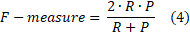
F-measure (also F-score or F1 score) is a measure of a test’s accuracy. The F-measure is the harmonic mean (average) of the precision and recall. F-measure is the best when precision (P) and recall (R) are balanced[25] In Table 2 is defined four types of model’s efficiency.
RESULTS
The initial data set is an Excel file that consists of 32 418 rows (instances) and 9 columns (items), among other things, studentID, academic year, courseID, and grade. The initial data set is transformed (pivoted). Final data set contains 1640 rows (studentID) and 169 columns, 5 columns for personal data and 164 (82 2 – date and grade) columns for courses. The data set covers 13 years. To speed up the data processing, for each model is created partial data sets extracted from the final data set. Partial data sets consist of grades of independent variables and dependent variables. The implementation of research is based on package GA. Package GA is not default package in R, so it is necessary to install. By command library(GA), users activate the package. RStudio is used as a GUI. Part of the code for Model 1 is given in Figure 1. Before the GA package activation, the data source was defined. Code line beginning with genetic (Figure 1) defines dependent (ocj_pred_4) and independent variables (ocj_pred_1, ocj_pred_2), and determines data source. Function ga is used for the maximization of a fitness function and function plot to create a diagram. The first step in the research is to analyze the correlation between grades of independent and dependent variables. Each variable consists of 6+1 grades, which means that the number of grades (parameters) in each model is multiplied by 7. For example, Model 1 has two independent variables and 2*7 = 14 independent sub-variables, 1 dependent variable, and 7 dependent sub-variables. Grades are 10, 9, 8, 7, 6, and 5 (not passed). Not participated is defined with 0.
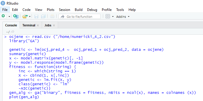
The second step in the research is to determine the level of success of the genetic algorithms as a method, and an adequate level of complexity determined by the number of independent variables. In Model 1 and Model 2 dependent variable is the same (course marked as ocj_pred_4), and the difference between these two models is the number of independent variables (Model 1 - two variables, Model 2 - three variables). The purpose of Model 1 and Model 2 is to compare the influence of increasing the number of independent variables to the model’s efficiency. Compared to Model 2, Model 3 and Model 4 have a 2 (3) times higher number of independent variables (Model 3 - 7 variables, Model 4 - 10 variables) and the purpose of Model 3 and Model 4 is to determine the influence of increasing the number of independent variables to the model’s efficiency. In all models, the number of iterations (generation) of the algorithm is 100, and it was performed through the training and test phase. Model 1 Model 1 was used to analyze the correlation between grades of ocj_pred_4 and 2 independent variables (courses), i.e., the correlation between 14 independent and 7 dependent sub-variables. In tables 3, 6, 9, and 12, the following tags are used: CourseID (CID), correlation coefficient (CC), P-value, level of statistical significance (LSS), and impact (Y/N) (I). List of courses: Independent variable ocj_pred_1 (CID 1) - Introduction to Information Technology ocj_pred_2 (CID 2) - Introduction to Operating System Dependent variable ocj_pred_4 (CID 4) - Project Management Note: CID – Course Identification number
All independent variables have satisfying values of correlation coefficients and an impact on the dependent variable. Independent variables have a positive direction.
| CourseID | 1 | 2 | |||||
|---|---|---|---|---|---|---|---|
| Correlation Coefficient | 0,299 | 0,488 | |||||
| p value | >0,000 | >0,000 | |||||
| Level of Statistical Significance | 1 | 1 | |||||
| Impact (Y/N) | Y | Y | |||||
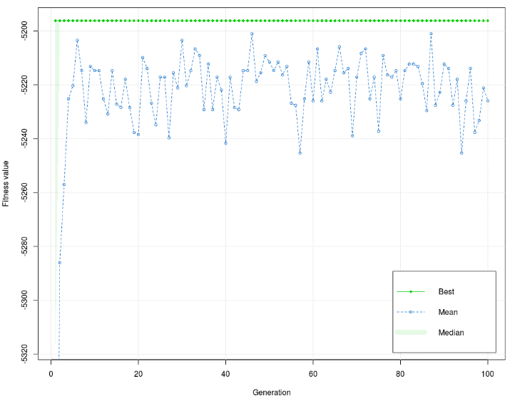
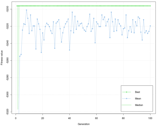
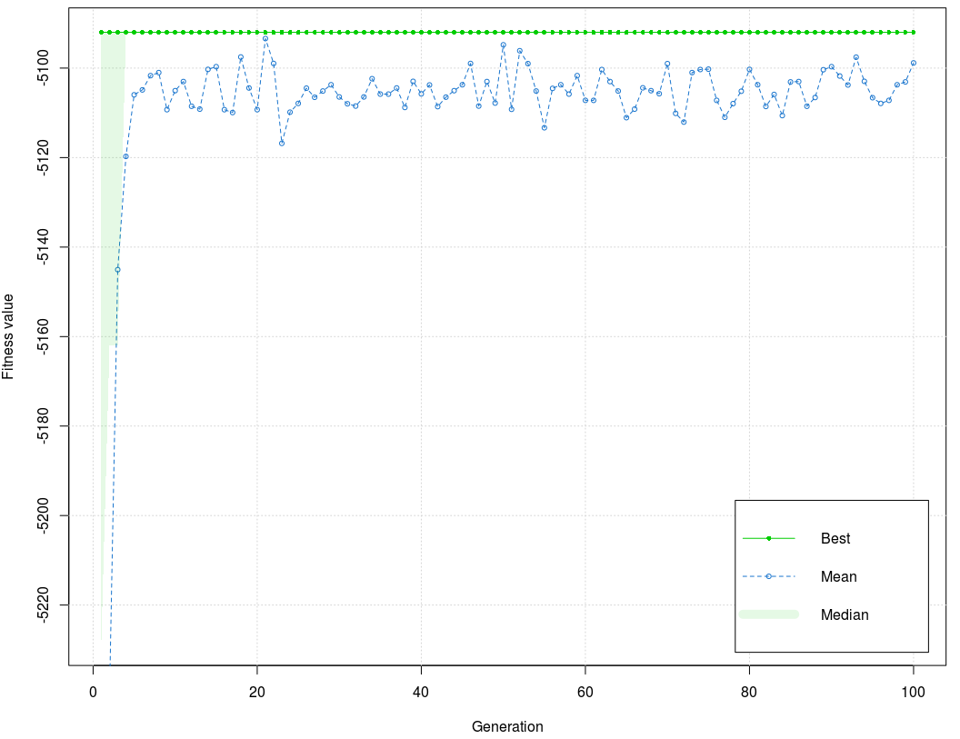
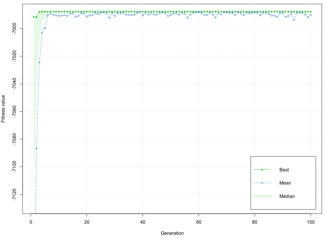
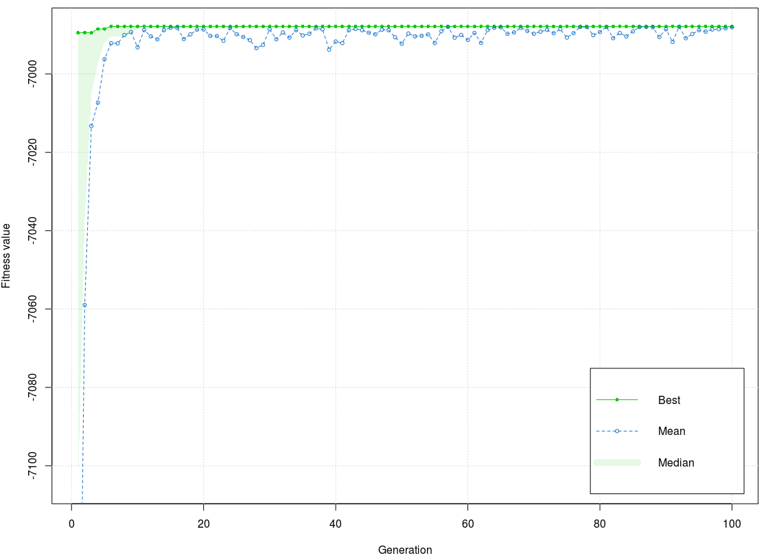
The best value of the fitness function is –5196,209, and the mean is –5203,471. Figure 2 shows that the values of the fitness function in the training phase are dissipated, but the interval is relatively low (40). Values on the graph are dissipated for early generations and stay until the end of the process, but, generally, it is concentrated around –5220. The graph has a few peaks, which are below –5240. Figure 3 shows that the values of fitness function are more dissipation, but the interval is still relatively low (50). As in the training phase, the graph has dissipated for early generations and stays that way to the end of the process, but, generally, it is concentrated around –5220. Unlike the training phase, more peaks are in the 1st half of the diagram, and the dissipations are larger. Although the diagram can indicate that the graph of the fitness function in the training and test phases has high dissipation, it causes the diagram scale. As mentioned earlier, the dissipation interval is relatively low. The best value of fitness function is the same in the test as in the training phase. Mean is lower than the mean in the training phase. Based on the graph in training and test phases, it is concluded that the mean in the test phase is more responding to the graph’s values in both diagrams.
Model 2 Model 2 was used to analyze the correlation between grades, of course, marked as ocj_pred_4 and 3 independent variables (courses), i.e., the correlation between 21 independent and 7 dependent sub-variables. All independent variables affect the dependent variable (Table 4). List of courses: Independent variables ocj_pred_1 (CID 1) - Introduction to Information Technology ocj_pred_2 (CID 2) - Introduction to Operating System ocj_pred_3 (CID 3) - Basics of Economics and Business Dependent variable ocj_pred_4 (CID 4) - Project Management Note: CID – Course Identification number
| CourseID | 1 | 2 | 3 | ||||||
|---|---|---|---|---|---|---|---|---|---|
| Correlation Coefficient | 0,227 | 0,356 | 0,356 | ||||||
| p value | >0,000 | >0,000 | >0,000 | ||||||
| Level of Statistical Significance | 1 | 1 | 1 | ||||||
| Impact (Y/N) | Y | Y | Y | ||||||
Compared to Model 1, correlation coefficients are lower, but ocj_pred_2 and ocj_pred_3 still have satisfying values of correlation coefficients. All independent variables have a positive direction. Figure 4 shows that the values of the fitness function in the training phase have dissipated, but the interval is low (35). Generally, the graph is stabilized and concentrated around mean for early generations and stays that way to the end of the process barring peaks before the 60th and 90th generation. The best value of the fitness function is –5091,995, and the mean is –5099,683.
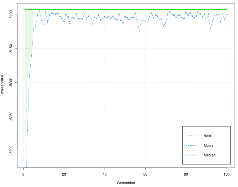
Figure 5 shows that the values of the fitness function in the test phase are less dissipating and that the interval is lower (20). As in the training phase, the graph is stabilized and concentrated around mean for early generations and stays as such to the end of the process with no important peaks. The best value of the fitness function is –5091,995, and the mean is –5098,838, a little bit higher than the training phase. Based on diagrams for the training and test phase, it is concluded that the test phase dissipation interval is lower (better) than the training phase. Model 3 Subsequent Model 3 was used to analyze the correlation between grades of ocj_pred_16 and 7 independent variables (courses), i.e., the correlation between 49 independent and 7 dependent sub-variables. List of courses: Independent variables ocj_pred_1 (CID 1) – Introduction to Information Technology ocj_pred_3 (CID 3) – Basics of Economics and Business ocj_pred_6 (CID 6) – Computer Systems Architecture ocj_pred_8 (CID 8) – English Language I ocj_pred_9 (CID 9) – Introduction to Databases ocj_pred_12 (CID 12) – English Language II ocj_pred_15 (CID 15) – Management and Information Systems Dependent variable ocj_pred_16 (CID 16) – Reporting Note: CID – Course Identification number Based on data presented in Table 5, it can be concluded that all independent variables have an impact on dependent variables. The highest impact (the highest absolute value) was course marked as ocj_pred_6, and the lowest (the lowest absolute value) was course marked as ocj_pred_12. Unlike Model 1 and Model 2, three independent variables have a satisfying correlation coefficient (>0,3). Other correlation coefficients are lower than 0,3, and two of them are close to 0,1. It can be concluded that the increase in the number of independent variables causes a decrease in values of correlation coefficients.
| CourseID | 1 | 3 | 6 | 8 | 9 | 12 | 15 | ||||||||||
|---|---|---|---|---|---|---|---|---|---|---|---|---|---|---|---|---|---|
| Correlation Coefficient | 0,153 | 0,254 | 0,433 | 0,125 | 0,372 | –0,108 | 0,345 | ||||||||||
| p value | >0,000 | >0,000 | >0,000 | >0,000 | >0,000 | >0,000 | >0,000 | ||||||||||
| Level of Statistical Significance | 1 | 1 | 1 | 1 | 1 | 1 | 1 | ||||||||||
| Impact (Y/N) | Y | Y | Y | Y | Y | Y | Y | ||||||||||
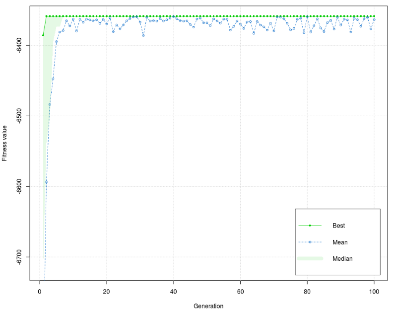
Figure 6 shows that there are two different forms of the best value of fitness function for the training phase, one for the 1st generation and the other for the next generations. The values of the fitness function are concentrated around 6375 in the low interval (<20) for early generations and stay the same to the end of the process. The best value of the fitness function is –6363,572, and the mean is –6358,652. The difference between the best value and the mean is very small, smaller than 5. Figure 7 shows that there are three different versions of the best value of the fitness function for the test phase (1st, 2nd, 3rd – 100th generation). Like the training phase, values of the fitness function are concentrated around 6375 in the low interval (<20) for early generations and stay the same to the end of the process. The best value of fitness function is almost equal to the training phase (–6363,953), and the mean is equal to the mean of the training phase (–6358,652). Distinct differences between the diagram of training and the test phase are in the form of a graph. The values of the fitness function in the test phase have low dissipation in the 1st and more balanced in the 2nd half of the graph. The training phase has an inverse manifestation. Furthermore, the training phase has a higher interval of dissipation. It can be concluded that the test phase dissipation interval is lower (better) than in the training phase. Model 4 Last Model 4 was used to analyze the correlation between grades of course marked as ocj_pred_22 and 7 independent variables (courses), i.e., the correlation between 70 independent and 7 dependent sub-variables. List of courses: Independent variables ocj_pred_1 (CID 1) - Introduction to Information Technology ocj_pred_2 (CID 2)- Introduction to Operating System
ocj_pred_4 (CID 4)- Project Management ocj_pred_5 (CID 5) - Mathematics ocj_pred_6 (CID 6) - Computer Systems Architecture ocj_pred_7 (CID 7) - Algorithms and data structures ocj_pred_8 (CID 8) – English language I ocj_pred_9 (CID 9) - Introduction to Databases ocj_pred_17 (CID 17) - Database management systems ocj_pred_18 (CID 18) - Statistics and probability Dependent variable ocj_pred_22 (CID 22)- Software engineering Note: CID – Course Identification number Based on data presented in Table 6, it can be concluded that two independent variables do not have an impact on a dependent variable. The rest of the variables have correlation coefficients lower than 0.2, and four variables have one lower than 0.1. Like Model 3, Model 4 has values of correlation coefficients lower than Model 1 and Model 2. The course marked as ocj_pred_8 has a negative direction. It can be concluded that a further increase in the number of independent variables causes a further decrease in values of correlation coefficients.
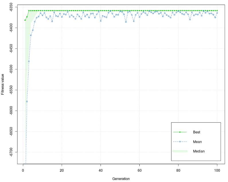
As Figure 8 shows, the training phase has two of the best values of the fitness function (1st - 2nd, 3rd – 100th generation). One part of the values is a little bit below the best, and the other part matches the best value of the fitness function. The interval is very low, and a few values are outside of it. The lowest value achieved was around the 95th generation. The best value of the fitness function is –6987,849 and mean –6990,114. The difference between the best value and mean is very small, smaller than 3.
As Figure 9 shows, the test phase has three of the best values in the function (1st-3rd, 4th-5th, 6th-100th generation). Unlike the training phase, the values of the fitness function have more dissipation. After the 60th generation, the values are stabilized and match the best value, but not like in the training phase. It can be concluded that the graph in the training phase is more stable. The best value of the fitness function is –6987,849 and the mean –6988,074. Differences between the best value and the mean are very low, lower than 3.
DISCUSSION – SUMMARY OF ALL 4 MODELS
Figures (2-9) show that values of the fitness function in Model 1 and Model 2 have higher dissipation. Unlike Model 1 and Model 2, dissipation in Model 3 and Model 4 is very low, i.e., the values are highly balanced. It can be concluded that an increase in the number of independent variables causes a decrease of dissipation and interval. Table 7 presents the number of correct and incorrect classified instances for all models. Models are marked as following: M1 – model 1, M2 – model 2, M3 – model 3, and M4 – model 4. Model 1 is set as a reference model.
| CLASSIFIED | M1 (2) | M2 (3) | I/Dv1(%) | M3 (7) | I/Dv2(%) | M4 (10) | I/Dv3(%) | ||||||||||
|---|---|---|---|---|---|---|---|---|---|---|---|---|---|---|---|---|---|
| Correct | 804 | 862 | 7,21 % | 1004 | 24,88 | 1214 | 51,00 | ||||||||||
| Incorrect | 836 | 778 | –6,94 % | 636 | –23,92 | 426 | –49,04 | ||||||||||
M1 (2) indicates Model 1 with 2 independent variables, M1 (3) indicates Model 1 with 3 independent variables, M3 (7) indicates Model 3 with 7 independent variables, and M4 (10) indicates Model 4 with 10 independent variables. I/D (%) indicates an increase/decrease of correct classified instances for model M2 (3) (I/Dv1), M3 (7) (I/Dv2), and M4 (10) (I/Dv3) regarding M1 (2) as a reference model. Based on data from Table 7, it can be concluded that the increase in the number of independent variables increases the number of correctly classified instances and decreases the number of incorrect classified instances. Table 8 presents the efficiency parameters by modules. M1 (2) indicates Model 1 with 2 independent variables, M1 (3) indicates Model 1 with 3 independent variables, M3 (7) indicates Model 3 with 7 independent variables, and M4 (10) indicates Model 4 with 10 independent variables.
I/D (%) indicates an increase/decrease of efficiency parameters for model M2 (3) (I/Dv1), M3 (7) (I/Dv2), and M4 (10) (I/Dv3) regarding M1 (2) as a reference model. Abbreviation I/D means Increase/Decrease of values of correct and incorrect classified instances (Table 7) and efficiency parameters (accuracy, precision, recall, F – measure - Table 8) by a number of independent variables. I/D values in Table 8 show that increasing independent variables don’t mean certainly increase in efficiency parameters. Table 8 shows that there is the optimal number of independent variables for which efficiency parameters have the best values. The reference model is model 1. Based on data from table 8, it can be concluded that: a) Based on values of efficiency parameters (35 % - 50 %) and the small difference between accuracy and the rest of the parameters, Model 1 is classified as type B. b) In Model 2, where the increase in the number of independent variables is small, values of correctly classified instances and all efficiency parameters increase. Based on the value of parameters which is in the interval 40 % - 50 % and small difference between accuracy and the rest of the parameters, it is concluded that Model 2 is classified as type B (same as Model 1), but has a smaller difference between efficiency parameters which means that it is better than Model 1. Namely, adding the variable ocj_pred_3 improves the number of correctly classified instances (approximately 60) and the accuracy (around 3 %). It can be concluded that adding one variable increase the method’s efficiency. c) Based on values of parameters that are on interval 30 % - 60 % and the large difference between accuracy and the rest of the parameters, Model 2 is classified as type C. Adding 4 variables improves the number of correctly classified instances (approximately 150) and the accuracy (about 10 %), but the values of the rest of the parameters decrease (-10). It can be concluded that adding 4 variables decreases correlation coefficients. d) Based on the values of parameters that are on the interval 20 % - 75 % and the large difference between accuracy and rest of the parameters, Model 4 is classified as type D. Adding 7 variables improves the number of correctly classified instances (approximately 350) and accuracy (about 25 %), but the values of the rest of the parameters decrease (–20). It is concluded that adding 7 variables decreases the method’s efficiency. e) In Model 3 and Model 4, where an increase in the number of independent variables is higher, values of correctly classified instances and accuracy increase, but values of precision, recall, and F-measures decrease. Model 3 has 7, and Model 4 has 10 independent variables. The percentage of decrease in precision, recall, and F-measures in Model 3 is approximately 30 % lower. In Model 4, I/D of the percentage of the interval is 30 % - 50 %. Consequently, it can be concluded that the increase number of independent variables has limitations because accuracy and three other efficiency parameters should be balanced as much as possible. Presented results show a large difference between accuracy and the rest of the parameters in Model 3 (2 times higher accuracy rate compared to the rest of the parameters) and especially in Model 4 (3.7 times higher accuracy rate compared to the rest of the parameters). Considering that, it is essential to balance the dissipation of values in the fitness function, balance the number of correct/incorrect classified instances, and the model’s efficiency. The results of the presented research indicate that the optimal number of independent variables should be between 3 and 7.
CONCLUSION
In this article, results prove that GA can be trained to provide a platform for predicting the success of students based on their already obtained grades. If we consider that each learning outcome builds over several different courses, GA can also be used to check the definition of learning outcomes in a given curriculum. Presented research shows that in Model 3 course marked as ocj_pred_8 (English language I) and course marked as ocj_pred_12 (English language II) as non-IT courses are in the last place on the scale level of statistical significance. It indicates an expected relation to several learning outcomes. Unlike Model 3, in Model 4, ocj_pred_8 is the course in 2nd class on the scale level of statistical significance that indicates an unexpected relation to several learning outcomes. That implies that the knowledge delivery process for the English language, including e-content, is latently related to IT skills and competences. This conclusion is significant because it shows that elements of learning outcomes (such as knowledge, skills, and competences) can be verified once there are enough grades in LMS. The practical implication of this article is using GA for the development of a more flexible knowledge delivery process, with data from modular (partial) examinations, by linking partial exam results to overall goals of one course. A huge problem for students is taking courses in which they have to develop skills and competences related to abstract thinking, as the learning curve proves to be too steep for many students due to several highly set goals. One of the standard solutions to that problem is to split the content into several modules dedicated to achievable goals. The limitations of this research are that it is primarily related to higher education in IT, and that is conducted at one HEI. Further research should investigate the use of GA in higher education in other fields (engineering, economy, social sciences, law, agriculture, and so on). Additionally, more HEIs should be included in the research to be able to confirm the efficiency of using GA for the development of a more flexible knowledge delivery process. Inefficiency or insufficient efficiency weakens the market position of a formal educational institution, i.e., managers, teachers, and students. The market position of the institution strongly defines personal market positions (managers, teachers, and students) and points to the strong dependence between all participants in the teaching process. Although they may seem less important, graduates are, in fact, the central figure of the entire teaching process, because they are its final product. In the final line, the more attractive HEI’s graduated students are in the job markets and the more successful they are in the workplaces (e.g., higher salaries, superior positions, increased responsibilities), usually, the higher is the rating of the particular HEI, as well as the rating of its managers and teachers.