
INTRODUCTION
The Traveling Salesman Problem (TSP) is one of the most extensively studied NP-hard graph search problems[1]. In the literature, there have been numerous published approaches for quality solutions, applying various techniques in order to find the optimum (least cost) or semi optimum solution. There are many different extensions and modifications of the original problem, such as The Time Dependent Traveling Salesman Problem (TDTSP)[2], this specific extension of the original TSP towards more realistic traffic conditions assessment. In the literature many researchers applied different methods in attempt of solving the TDTSP[3]. Here we propose a novel approach using fuzzy numbers, since we look at the jam regions and rush hours as uncertain factors that cannot realistically be represented with crisp numbers. In 1965, fuzzy sets as an extension of classical notion of set were introduced by L.A. Zadeh[4]. According to that, membership functions ranging in the unit interval [0, 1] can help to describe such phenomena as uncertain extension of the jam region (an uncertain sub-graph of the original complete graph), and the uncertain timely extension of the rush hour period, more efficiently. On the other hand, there are several generalizations of fuzzy set theory for various objectives; the notion of intuitionistic fuzzy sets (IFSs) introduced by Atanassov[5] is an interesting and useful one. Fuzzy sets are (special) IFSs but the converse is not accurately true[6]. In fact, there are situations where IFS theory is more convenient to deal with[7]; the TDTSP with jam factors is a prime example. In addition, it has been shown by several researchers that realistic sets with uncertainty factors may be properly modelled by IFSs. IFS theory has been applied in different areas that have to do with decision making under high hesitation and vagueness degrees and it prove being successful. In the present article we study the extended TDTSP problem using the notions of IFS theory by introducing the broadened model.
THE INTUITIONISTIC FUZZY TIME DEPENDENT TRAVELING SALESMAN PROBLEM (IFTD TSP)
In the TDTSP the goals is to calculate the time required to cover the distance between cities is vital. Since the cost elements are time dependent, then the actual cost between two cities can be determined only if the total time elapsed is precisely resolved. Considering an actual salesman tours, especially in city centres, the topography and rush hours in variant locations are factors that must be looked at as uncertain or vague values, more precisely as fuzzy numbers. Hence, relevant data for estimated tour distance between two nodes is not constant as suggested previously In the classic TDTSP[2]. On the contrary, it can be more appropriate to represent this imprecision using the intuitionistic fuzzy model. This in turn will introduce more realistic trips measurements and ultimately optimized solution for TDTSP problem with traffic jam factors. In the following section we will go through some definitions before we apply our propsed model on a sample tour and prove its efficiency. DEFINITIONS Let us start with a short review of basic concepts and definitions related to intuitionistic fuzzy sets which are used in the upcoming sections. DEFINITION 1 Let a universal set E be fixed. An intuitionistic fuzzy set or IFS A in E is an object having the form

where
The amount

is called the hesitation part, which may cater to either the membership value or to the non-membership value, or to both. DEFINITION 2 Let E be a nonempty classical set and let A and B be intuitionistic fuzzy sets of E, then

if and only if
if and only if


if


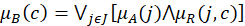
where Ac is the complement of A. DEFINITION 3 Let X and Y be two nonempty classical sets. An intuitionistic fuzzy relation (IFR) R from X to Y is an IFS of X × Y, characterized by the membership function μR and the non-membership function v_R. An IFR R from X to Y will be denoted by R(X→Y). DEFINITION 4 If A is an IFS of X, the max-min-max composition of the IFR R (X → Y)with A is an IFS B of Y denoted by (B = R∘A); and is defined by the membership function

and the non-membership function


DEFINITION 4 Let Q(X → Y) and R(Y → Z) be two IFRs. The max-min-max composition (R ∘ Q); is the intuitionistic fuzzy relation from X to Z, defined by the membership function

and the non-membership function given by


IFTDTSP In the TSP, the salesman originally attempts to find the optimal (shortest) route starting from the initial node (company headquarters), so that all nodes (cities, shops or other locations on the agenda) are visited exactly once and then returns to the starting point[1]. We suppose E is a set of edges; where the edge is the distance between two nodes as shown in (Figure 1). Each edge possesses a fuzzy jam factor due to the topography of the paths between cities (nodes). C is the set of jam factor costs (for short we will refer for it from now on as costs). We define an intuitionistic fuzzy relation R from the set of jam factor J to the set of C (i.e., on J × C) which reveals the degrees of association and of non-association between jam factor and cost. There are three main steps that formulates the core of our IFTSTSP model: 1. Determination of edges that have jam factors. 2. Formulation of cost knowledge based on intuitionistic fuzzy relations. 3. Determination of cost on the basis of composition of intuitionistic fuzzy relations. Let A be an IFS of the set J, and R be an IFR from J to C. Then the Max-Min-Max composition as in Equations (8) and (9), B of IFS A with the IFR R(J → C) denoted by B = A ∘ R signifies the cost of the edges as an IFS B of C with the membership function given by
and the non-membership function given by
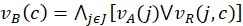

If the state of the edge E is described in terms of an IFS A of J; then E is assumed to be the assigned cost in terms of IFS B of C, through an IFR R from J to C, which is assumed to be given by knowledge base directory (or experts who are able to translate the jam degrees of association and non-association according to geographical areas) on the destination cities and the extent (membership) to which each one is included in the jam region. This will be translated to the degrees of association and non-association, respectively, between jam and cost. Now let us expand this concept to a finite number of edges E that form a whole tour for a salesman. Let there be n edges Ei; i = 1, 2, ..., n; in a trip (from starting point to final destination). Thus


and construct an IFR Q from the set of edges E to the set of jam factors J. Clearly, the composition T of IFRs R and Q
give the cost for each edge from E to C given by the membership function

and the non-membership function given by

For given R and Q, the relation

can be computed. From the knowledge of Q and T, an improved version of the IFR R can be computed, for which the following statements are valid:
is maximal, ii) The equality 𝑇=𝑅∘𝑄 is retained
Clearly, this improved version of R will be a more significant IFR translating the higher degrees of association and lower degrees of non-association of J as well as lower degrees of hesitation to the cost evaluation C. If almost equal values for different C in T are obtained, then we consi- der the case for which hesitation is least. From a refined version of R one may
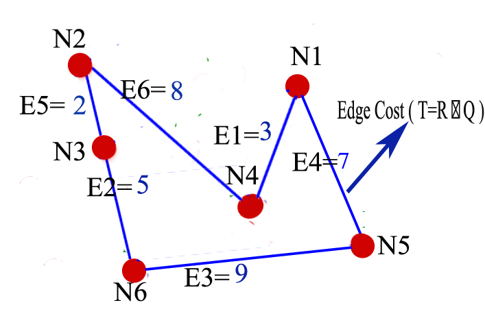
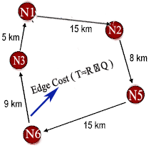
infer cost from jam factors in the sense of a paired value, one being the degree of association and other the degree of non-association. APPLICATION ON A SIMPLE TDTSP CASE Let there be a tour that has only 6 edges (edge 1. – edge 6) as shown in (Table 1). Each edge connects two nodes (Figure 1). Thus, each edge eventually will have a jam cost, depending on the area(s) it crosses. (Table 1) shows each edge and the jam factors associated. The ultimate goal is to be able to calculate the total tour jam factor which will be multiplied in the physical distance between two nodes. Hence, quantifying the jam cost for each edge that is part of that tour path. The intuitionistic fuzzy relation

is given as shown in (Table 1). Let the set of jam costs be C as in Table 2. The intuitionistic fuzzy relation

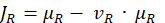
as in Table 2. Therefore the composition

as given in Table 3. We calculate JR (Table 4). Hence, those numbers quantify the jam factor on each edge. After a simple calculation

we obtain the actual cost for each tour accumulating the edges after multiplying the physical distances with the jam factors in (Table 4).
CONCLUSIONS AND FUTURE WORK
In this article, we proposed a novel intuitionistic fuzzy set based model for the realistic extension of the TDTSP, namely, the IFTDTSP model, for considering the jam factors in the original TDTSP problem by applying the IFS theory. Obviously, this improved version will be a more promising approach in translating the higher degrees of association and lower degrees of non-association of jam factor as well as lower degrees of hesitation to any edge’s cost and ultimately more realistic calculation for the traveled routes. Our future work will focus on applying the DBMEA meta-heuristics[8][9] for determining the (quasi) optimal tours (as this algorithm has been repeatedly successfully applied for various NP-hard graph search problems with rather good accuracy, very good predictability and rather universally) to our model and test its efficiency on larger number of nodes.