
INTRODUCTION
In recent years incredible progress in the field of artificial intelligence, machine learning and neural networks has been seen. Machine learning, as a subset of artificial intelligence, is closely related to computational statistics related to the building of algorithms which learn on training data to make predictions. It is is a current application of artificial intelligence concerned with the discovery of models, patterns and other regularities in data[1]. Machine learning is one of the most exciting recent technologies in artificial intelligence and has many applications that’s we make use of daily such as virtual personal assistants, videos surveillance, social media services, online customer support, etc.[2]. Machine learning algorithms have become a very popular tool for analysing financial data and forecasting stock prices in the last few years[3]. The rapid growth of information technology and the Internet lead to the fast development of computer science methods. Neural networks are efficient methods for stock market prediction mostly implemented in forecasting stock prices and returns. The backpropagation algorithm is most frequently methodology used. The benefits of the artificial neural network are their ability to predict stock price movements even in situations with uncertain data[4]. The prediction of stock market prices and indexes is, however, a difficult task because various factors affect the stock price formation. The goal of this article is to forecast stock market indexes using machine learning algorithms. Weka is a collection of machine learning algorithms for various data mining tasks such as data pre-processing, classification, regression, clustering, associate rules, visualization and forecasting. The algorithms are Linear regression, Gaussian Processes, SMOreg and neural network Multilayer Perceptron. In the article, the prediction of five major stock market indexes (DAX performance-index (DAX), Dow Jones Industrial Average (Dow Jones), NASDAQ Composite (NASDAQ), Nikkei 225 and S&P 500) will be made using historical data from February 1, 2010, to January 31, 2020. The prediction will be made separately for each of observed major stock market indexes using historical (training) data for three different periods (ten, five and one years) using machine learning algorithms. The forecast will be made for 5, 10, 15 and 20-time units (days) in the future. In that way, it will be inspected how well selected forecasting approaches are performing for different forecasting horizons. The forecasting precision of machine learning tools will be evaluated using MAE, MSE and MAPE error metrics. It is expected that machine learning algorithms will have a high level of precision in predicting the future values of major stock market indexes. The novel in this article in regards to the previous research is more rigorous analysis of stock market indices forecasting using machine learning algorithms. In the article the comparison of machine learning algorithms’ efficiency was made using historical training data on a longer and medium time period (10, 5 and 1 year) and by deviding the evaluations on training and held-out training 0,3 data for five stock market indices (DAX, Dow Jones, NASDAQ, Nikkei 225 and S&P 500). The robustness of the analysis is evident in using various error metrics (MAE, MSE and MAPE) for evaluation of forecasting precision of machine learning algorithms in five, ten, fifteen and twenty day horizon forecasts in the future. In this way the efficiency of machine learning algorithms was examined in a more comprehensive way in regards to the previous research. Article is structured in five chapters. After the introduction, literature review elaborates on the application of machine learning techniques in stock market prediction. In the methodology and data section, the main characteristics of data and data sources are explained. Besides, the preparation of data for the analysis in a detail are explained the main features of machine learning algorithms. In the results and discussion section, descriptive statistics of data is displayed first after which the individual forecasting performance for the market indices and comparison of forecasting results between the market indices is presented. The final chapter presents concluding remarks, gives limitations of article and guidelines for future research.
LITERATURE REVIEW
In[5] built a model using a decision tree classifier and historical data of three major companies listed in the Amman Stock Exchange (ASE). The proposed model could be a helpful tool for investors in the stock market to decide when to buy or sell stocks. The stock market price prediction ability of artificial neural networks before and after demonetization in India[6] by observing nine stocks and CNX NIFTY50 index was investigated. Multilayered neural networks were trained by the Levenberg-Marquardt algorithm. The networks proposed efficiently predicted the close price and worked best for high volatile market conditions. A predictive study of the principal index of the Brazilian stock market[7] with the help of artificial neural networks and adaptive exponential smoothing method was performed. The objective was to compare the forecasting performance of both methods by evaluating the accuracy of both methods to predict stock market returns. The results showed that both methods produced similar results in predicting the index returns. In[8] the ensemble learning algorithm to increase predictive efficiency developed. Twelve indicators are ranked by market participants using the VIKOR method. The importance of each indicator was based on specified nose and output values. The results have shown that OBV, CCI and EMA indicators are very important. Furthermore, the SVM method of machine learning showed the superiority of the results in prediction accuracy. Using Rapidminer tool[9] examined and applied different prediction models techniques using stock market historical prices giving recommendations for buying or selling in the stock market. Comparing different predictive functions they found that deep learning function predicted stock price more accurately than other functions. According to[10] different techniques for stock prediction were classified categorically in time series, neural network and its variations and hybrid techniques (the combination of neural network with different machine learning techniques). It was shown that the neural network was the best technique to predict stock prices, especially in the case when de-noising schemes are applied with the neural network. Five methods of analyzing stocks to predict day’s closing price[11] were combined. Those are Typical Price (TP), Bollinger Bands, Relative Strength Index (RSI), CMI and Moving Average (MA). The results showed that algorithms predicted closing price in more than 50 % of cases with a high level of significance. Recurrent neural networks with character-level language model pre-training for both intraday and interday stock market forecasting were explored[3]. It was shown that the use of character-level embeddings was promising and competitive with other complex models which use technical indicators and event extraction methods. The authors[12] predicted the Turkish stock market BIST 30 Index using deep learning where features are selected from common important technical indicators. They trained and tested their model to outperform other techniques such as an artificial neural network (ANN) concluding that deep learning has proved itself as a promising solution for complex problemsolving. A comprehensive survey of more than 150 articles on machine learning application to financial markets forecasting was made[13]. Machine learning algorithms tend to outperform traditional stochastic methods in financial market forecasting. Moreover, on average recurrent neural networks outperformed feed-forward neural networks as well as support vector machines.The profitability of artificial neural networks on the Taiwan Weighted Index and in the S&P 500 was investigated[14]. The authors created an efficient and inexpensive method for investors to ensure a good investment return and found that the trading rule based on artificial neural networks generates higher returns than the buy-hold strategy. Neural networks to forecast S&P and Gold futures in the period of 90 months were employed[15]. The forecasted parameters for the networks relied on 15 months of patterns while network forecast performance was tested and evaluated over a period of 75 months. The networks were able to correctly predict the sign of the price change in 61 % and 75 % of the times for gold trade and the S&P index. A method of feature selection for stock indexes and deep learning model to do sentiment analysis was proposed[16]. An accurate stock trend prediction method chosen was LSTM (Long Short-term Memory). Two approaches for measurement and forecasting of realized variance are Heterogeneous AutoRegressive model (HAR-RV) and Feedforward Neural Networks (FNNs),[17]. The application was made for the DAX index. Compared to traditional models FNN-HAR-type models had better accuracy but only on the sample data. Conditional Value-at-Risk (CVaR) method was applied for the Croatian stock market on th sample of 29 stocks grouped into 8 sectors in three different periods. The results have shown that sectors that are risky in the period of economic growth are not the same sectors that are risky during the period of economic crisis or stagnation,[18]. In this article a comprehensive approach for forecasting of stock market indices will be made by applying machine learning algorithms. The methodology applied in the article builds on previous attempts in the empirical literature by imploying a comprehensive and extensive approach to analysis of major stock market indices. The comparison of machine learning algorithms’ efficiency was made by using longer historical time-data series for five stock market indices, dividing the data on training and held-out training dataset, expanding the forecast horizon from five to twenty days and implementing different error metrics (MAE, MSE and MAPE).
DATA AND METHODOLOGY
Following the research aim of the article to forecast major stock market indexes using machine learning techniques and in order to inspect the successfulness and usability of different forecasting approaches, two main requirements should be fulfilled. The first requirement is the availability of long enough time series. The second requirement is that there are no many time series breaks or periods with no data availability. In order to meet both criteria, it has been decided that in the article data related to five major world market indices are going to be observed and analysed. Following five market indices are chosen: DAX performance-index (DAX), Dow Jones Industrial Average (Dow Jones), NASDAQ Composite (NASDAQ), Nikkei 225 and S&P 500. The data for the selected market indices are taken from the Yahoo! Finance web page[19][20][21][22][23]. Despite the fact that all data are taken from the same source, the observed market indices values are given in the national currencies. So, DAX is given in euros, Dow Jones, NASDAQ and S&P 500 are in US dollars, whereas Nikkei 225 is given in yens. The analysis in the article is based on historic data of various lengths. The reason for using historic time series data of different lengths is to inspect the accuracy of used forecasting approaches when a different number of training data is used as a base for calculating forecasts. Overall, three database periods are observed in the article: long, medium and short. The long base period includes historical data for the period of 10 years, the medium base period includes data for five years, whereas the short base period includes historical data from just one year. Here the 10 years base period covers historical data from February 1, 2010, to January 31, 2020, the five years base period includes data from February 1, 2015, to January 31, 2020, and the one-year base period includes historical data from February 1, 2019, to January 31, 2020. It has to be emphasized that in the article daily close prices adjusted for splits are observed only. For the analysis, the data are converted from .xls and .csv formats into .arff format. The process of preparation of DAX index data for .arff format is presented in a few rows of commands in Figure 1.
@relation DAX
@attribute date date "yyyy-MM-dd"
@attribute close numeric
@data
2010-02-01,5654.479980
2010-02-02,5709.660156
2010-02-03,5672.089844
2010-02-04,5533.240234
2010-02-05,5434.339844
…
2020-02-01,13204.76953
2020-01-28,13323.69043
2020-01-29,13345.00000
2020-01-30,13157.12011
2020-02-02,12981.96972
Figure 1. Preparation of DAX stock market index data.
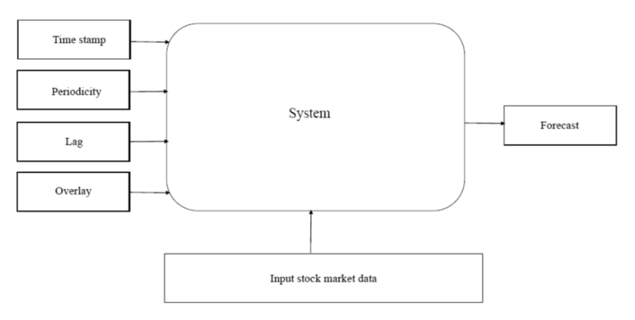
In Figure 2 is illustrated system framework for major stock market indexes prediction containing input stock market data, timestamp, periodicity, lag and overlay which are inserted into the system to forecast data.
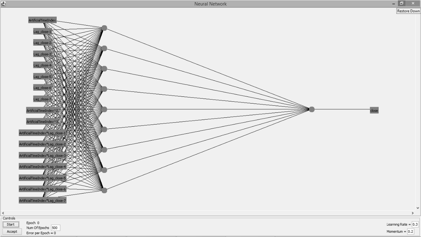
The process of forecasting is conducted in Weka, version 3.8.4 software[24] with installed timeseriesForecasting package version 1.0.27[25]. In the basic configuration window, it has been chosen that 5, 10, 15 and 20-time units (periods) should be forecasted in the future. In that way, it will be inspected how well selected forecasting approaches are performing for different forecasting horizons. As a timestamp the option „Use an artificial time index“ is used but under periodicity, the option „Daily“ is selected. Under the advanced configuration window, four base learner configurations or four different forecasting approaches are selected. To enable comparability and repeatability of the research default settings of the base learner configurations are used. Following four base learner configurations are used: Gaussian processes for regression (Gaussian processes), linear regression for prediction (Linear regression), the backpropagation to learn a multi-layer perceptron to classify instances (Multilayer perceptron) and support vector machine for regression (SMOreg).Gaussian process for regression is a Bayesian or nonparametric approach to regression which becomes often used in the area of machine learning[26]. When the Gaussian process for regression is applied, the prior of the Gaussian process should be specified. Here the prior mean is assumed to be equal to the training data’s mean. On the other hand, linear regression is one of the most commonly used traditional predictive models[27]. In the linear regression models, the association between the output variable and explanatory variables is assumed to be estimated with a linear line. It is assumed that the distances of actual data values and the regression line is minimized. Here the simple linear regression model is assumed in which output variable is the close price of an observed market index whereas the explanatory variable is time. The multilayer perceptron is a supervised learning algorithm that learns by training on a dataset. A multilayer perceptron has consisted of an input layer and an output layer. Between those two layers, it can be found one or more nonlinear layers which are called hidden layers.
The backpropagation is a learning algorithm which is often used at multiplayer perceptron for finding the minimum error function. A detailed explanation of steps in multilayer perception with a hidden layer is shown in[28]. The sequential minimal optimization (SMO) is an iterative algorithm for solving regression problems by using support vector machine proposed by[29]. The analysis is conducted in two ways. The first way is to include all data as base or training data. In a second way, 30 % of the training data has been held out from the end of the series to form an independent test set. To evaluate used forecasting approaches following forecasting errors are used: mean absolute error (MAE), mean squared error (MSE) and mean absolute percentage error (MAPE). All forecasting errors are calculated by observing actual and forecasted values in the certain forecast horizon (5, 10, 15 or 20 days). By observing forecast errors in different forecast horizons, it will be inspected how the precision of a certain forecasting approach is changing with the change in the forecast horizon. In that way, it will be possible to conclude whether it is appropriate to use certain forecasting approach for forecasting more periods in the future or should it should be used only for short forecasting horizons.Mean absolute error is calculated as an average of absolute differences between actual and forecasted values. Mean squared error takes into account an average of squared differences of actual and forecasted values. Mean absolute percentage error is calculated as an average of absolute differences between actual and forecasted values divided by actual values and multiplied by 100. Because the observed market indices are not all given in the same units, mean absolute error and mean squared error are going to be used to evaluate forecasting approaches for each market index separately. On the other hand, the mean absolute percentage error is going to be used to compare results between the market indices as well. In Equations 1-3 are presented formulas for calculation of MAE, MSE and MAPE values.
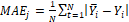
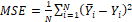
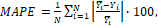
where ӯi is the predicted value and Yi is the observed value for the number N of observations. In Table 1 the interpretation of MAPE values according to the range of observed errors is explained.
| MAPE value | Interpretation | ||
|---|---|---|---|
| <10 | 9 377* | ||
| 10-20 | Good forecasting | ||
| 20-50 | Reasonable forecasting | ||
| > 50 | Inaccurate forecasting | ||
The value of MAPE lower than 10 can be interpreted as highly accurate forecasting, the value of MAPE in the range of 10-20 can be interpreted as good forecasting, the value in the range of 20-50 is reasonable forecasting while the value of MAPE higher than 50 can be interpreted as inaccurate forecasting.
RESULTS AND DISCUSSION
DESCRIPTIVE STATISTICS The close values of the five market indices (DAX, Dow Jones, NASDAQ, Nikkei 225 and S&P 500) are observed in three different periods. Therefore, three descriptive statistics analyses have been conducted. The descriptive statistics results are shown in Tables 2, 3 and 4. In Table 2 descriptive statistics results by observing a period of 10 years is given whereas in Table 3 descriptive statistics results are given by taking into account period of 5 years. In Table 4 descriptive statistics results are presented for taking into account close daily values of the observed market indices in the period of one year. The descriptive statistics analysis results, which are given in Table 2, include close daily values in the 10 years from 1.2.2010 to 31.1.2020. Therefore, those results are presenting the situation in the long term. Due to a different number of working days, the count of daily data is different among the observed market indices. However, there are no large differences in the data count between the given market indices. Still, the coefficients of variation values reveal that in the long term the close daily prices of market indices have high variability (or volatility) level. The highest variability level in the observed period had NASDAQ (41 %) whereas the lowest variability level had DAX (25 %). The distributions of close daily prices for stock market indices DAX, Nikkei 225 and S&P 500 seem to be approximately symmetric whereas data distributions of Dow Jones and NASDAQ seem to be weak and positively asymmetric. All five observed data distributions are flatter than the standardized normal distribution is.
The descriptive statistics analysis results, given in Table 3, are calculated based on close daily market indices values in the period from 1.2.2015 to 31.1.2020. The results are showing that the variability level of close daily prices is much lower in this 5-year period than in the 10-year period. The lowest variability level in this 5-year period had DAX (9 %) whereas the highest variability level had Nikkei 225 stock market index (25 %). All observed stock market indices had distributions of close daily prices almost symmetric expect DAX index for which data distribution is weak and negatively asymmetric. As in the 10-years period, all data distributions are flatter in comparison to the standardized normal distribution. In Table 4 the results of the descriptive statistics are given for the period of just one year where the close daily prices are observed from 1.2.2019 to 31.1.2020. In this short term,
coefficients of variation values are showing that close daily prices have low variability for all five observed market indices. However, all five data distributions of close daily prices are more skewed than they were in the medium (5 years) and long-run (10 years). Only the distribution of close daily prices for NASDAQ stock market index is less flat than the standardized normal distribution whereas the other four data distributions are flatter. INDIVIDUAL FORECASTING PERFORMANCE FOR THE MARKET INDICES In this chapter for each observed stock market index the most precise forecasting approach is emphasized. The best forecasting approaches are listed separately according to the mean absolute error and the mean squared error criteria. In other words, in Tables, A1-A5 in the Appendix are given forecasting approaches for which the lowest error values for different situations are achieved. The best forecasting approaches are listed by taking into account forecast horizons of 5, 10, 15 and 20 days. Furthermore, base period lengths of 1, 5 and 10 years have been taken into account as well. Finally, the fact of whether all historic data or just 70 % of them has been involved in the calculation of forecast values has been also observed. It has to be emphasized that the exact results of mean absolute errors and mean squared errors are not given here due to article length limitations but the data are available upon request. In Table A1 in Appendix the best forecasting approaches for DAX are given. Both observed errors, mean absolute error and mean squared error, led to the choice of the same forecasting approach in all cases but the last one. If all data are used to calculate forecasts, SMOreg approach has shown to be the best solution if data from 10 years are observed. On the other hand, multilayer perceptron turned out to be the most precise forecasting approach when data only from one year are observed. If 30 % of the training data has been held out from the end of the series, it turned out that linear regression is the most precise when data from 10 years are used, multilayer perceptron is the best solution for time series of 5 years, whereas SMOreg is the most appropriate for short time series with a length of one year. In Table A2 in Appendix the best forecasting approaches for Dow Jones are listed. It has been shown that, when all data are observed, multilayer perception is the most precise forecasting approach when the base period length is 5 and 10 years. However, this is valid only if the forecast horizon is shorter than 20 days. On the other hand, when 30 % of the training data has been held out from the end of the series SMOreg turned out to be the most appropriate forecasting approach in most cases. According to the results from Table A3 in Appendix, where the best forecasting approaches for NASDAQ are shown when all data are observed, multilayer perception is the best solution when forecasts are based on a long period (10 years), SMOreg for the medium-long period (5 years) and Gaussian processes for short period (one year). When 30 % of the training data has been held out from the end of the series, Gaussian processes turned out to be the most precise forecasting approach for short period whereas in other situations SMOreg seems to be the best choice. Table A4 in Appendix contains a list of best forecasting approaches for Nikkei 225. When all data are used, it can be concluded that SMOreg is the best forecasting approach when forecasts are based on data from medium-long period. However, no other pattern can be recognized. On the other hand, when 30 % of the training data has been holding out from the end of the series, Gaussian processes turned out to be the most precise forecasting approach when forecasts are based on data from the short period (one year), SMOreg for forecasts based on data from the medium-long period (5 years) and linear regression is the best solution for forecasts based on data from the long period (10 years). In Table A5 in Appendix the best forecasting approaches for S&P 500 are listed. It turned out that, when all data as a base for forecasts are used, multilayer perceptron is the best solution when forecasts are based on data from the long period (10 years). In other cases, Gaussian processes approach seems to be the most precise. On the other hand, when 30 % of the training data has been holding out from the end of the series, Gaussian processes turned out to be the most precise forecasting approach when forecasts are based on data from the short period (one year), linear regression is appropriate for forecasts based on data from the medium-long period (5 years) and linear regression is the best solution for forecasts based on data from the long period (10 years). COMPARISON OF FORECASTING RESULTS BETWEEN THE MARKET INDICES To compare the best forecasting approaches between the observed market indices, the mean absolute percentage error was used. The main reason for that can be found in the fact that not all observed market indices are given in the same units (US dollars, euros, yens). In this way, the direct comparison between the observed market indices can be made. In the following tables, Tables 5-10, mean absolute percentage error values for the observed market indices for different base period lengths (1, 5 and 10 years) are given. Besides, the demarcation between situations when all data as base or training data are used and when 30 % of the training data has been holding out from the end of the series is observed as well. In the aforementioned tables, the lowest values of mean absolute percentage errors for each observed market index and four forecast horizons are bolded.
According to the results from Table 5, it can be concluded that multilayer perceptron should be used as the most precise forecasting approach when long base periods are used. However, this choice is justified only for short forecast horizons. Furthermore, it should be mentioned that this conclusion is valid for four out of five observed market indices. Namely, in this case, SMOreg turned out to be the best choice for forecasting DAX.
In Table 6 base period length is reduced from 10 to 5 years and conclusions became not so straightforward. For NASDAQ and Nikkei 225 the most precise forecasting approach turned out to be SMOreg whereas for Dow Jones that is multilayer perceptron and for S&P 500 Gaussian processes. Those conclusions remained the same for all four observed forecast horizons. By reducing the base period length to one year the general conclusion is even more difficult to bring. The results from Table 7 are not consistent across the observed market indices. In the short forecast horizons, Gaussian processes and SMOreg forecasted well. However, for longer forecast horizons multilayer perceptron turned out to be the most precise forecasting approach. In Table 8 the values of mean absolute percentage errors are given when the base period length is 10 years but when 30 % of the training data has been holding out from the end of the series. The results are consistent through all forecast horizons. For Dow Jones, NASDAQ and S&P 500 the most precise forecasting approach is SMOreg whereas for DAX and Nikkei 225 the most precise forecasting approach is linear regression.
According to the results from Table 9, when the base period length is reduced to 5 years, SMOreg forecasting approach turned out to be the most precise in most cases through all four observed forecast horizons. When the base period length is reduced to one year and when 30 % of the training data has been holding out from the end of the series, the results from Table 10 are suggesting that Gaussian processes should be used as the most precise forecasting approach. However, for forecasting DAX the most precise forecasting method turned out to be SMOreg. From the aforementioned results, it can be concluded that machine learning algorithms achieved highly accurate forecasting performance although in some cases the precision could be classified as good forecasting. The exception is the Gaussian processes which showed some incompatibility with data predicted. However, the precision of this algorithm was better for shorter base period lengths and forecast horizons, ie. 1 year base period and 5 days forecast horizon. The precision of all algorithms was expectedly better for shorter base periods and shorter forecast horizons. Furthermore, the precision of all algorithms was much better when all data were included in the analysis concerning the evaluations based only on 0,3 training data. Results obtained from this analysis are in line with other research in this field, machine learning algorithms and neural networks can be characterized as efficient methods for stock market index prediction.
CONCLUSIONS
The goal of the article was to forecast stock market indexes using machine learning algorithms. The results of the analysis have shown that machine learning algorithms achieved highly accurate forecasting performance but in some cases, Gaussian processes specifically, the precision was less than high accurate. This could be explained with the algorithm’s incompatibility
with data predicted. The overall precision of all algorithms was better for shorter base period lengths and shorter forecast horizons as well as when all data were included in the analysis regarding the evaluations based on only on 0,3 training data. Limitations of the article are related to the use of only historical data for the prediction of stock market index values. This is, however, the most common approach in forecasting stock price movements. The use of historical data corresponds to the technical analysis of the stock market. Technical analysis studies historical market data, including prices and volumes in the form of chart patterns and technical indicators. In this article, the fundamental analysis was left out of the framework. Another important limitation of the use of machine learning algorithms for prediction of stock market indexes is in the case of unexpected events or Black swan events such as the spread of COVID-19 when the precision of forecast could not be the most accurate. The achieved performance of machine learning algorithms evaluated in this article could be improved with the inclusion of fundamental analysis as a measure of security’s intrinsic value by examining related economic and financial factors. Recommendations for future research could be related to further optimization of algorithms used and investigation of COVID-19 impact on stock market indexes. Stock price prediction remains one of the most complex issues in finance because the factors that influence stock price formation are complex and hard to predict. The optimal prediction method based on machine learning algorithms could help investors in determining their actual best buy-sell strategy and maximizing their profit.