
INTRODUCTION
The mountain regions scattered across the Earth’s crust are unique due to altitude and slope. Namely, the most common features in mountain areas are the steepness and ruggedness1. Throughout history, these features have significantly affected some countries (environmentally, socially and economically)2. Mountain areas occupy slightly less than one third of the global land area3; they provide essential ecosystem goods and services (EGS) for both mountain dwellers and people living outside these areas4. The decline of extractive industries such as mining, logging and farming and limited economic table-wrap have prompted many such regions to redirect development towards tourism for diversification2. As one author remarked, greenhouse gasses (GHG) removal strategies go hand in hand with: afforestation, reforestation, and management changes5. Interventions to reduce GHG in mountain regions are predominantly needed having in mind that these regions are hotspots and cradles for biodiversity3, serving as providers of myriad ecosystem services (ES) essential for humans including: carbon sequestration, air quality purification, water provisioning, food producing, tourism and recreation supply6-8. This article will deepen the research agenda on reducing GHG emissions, by examining the effect of Metropolitan Public Gardens Association (MPGA) legislative regulation to prevent environmental degradation with a specific focus on three environmental quality indicators: carbon dioxide (CO2), methane (CH4) and nitrous oxide (N2O). To slow the environmental devastation linked to global warming, MPGA countries implemented interventions to reduce GHG, with varying intensity. The praxis so far suggests that environmental policy conditions (e.g. public laws and regulations) can be counteracting forces in achieving operational integration goals which are directed at reducing GHG and making the mountain landscape more environmentally resilient. Special consideration is given to interventions related to agriculture, urbanisation and nature conservation. Environmental pollution is strongly controlled by specific legislation, which has led to prudent investments in environmental control. The main research question addressed in this article is: have environmental regulations helped these countries to reduce their GHG footprint? Or, in other words, having in mind that information on legislation or contents at a micro-level is unavailable to us, have the countries that entered into the MPGA observed a reduction in the three aforementioned environmental quality indicators? In addressing these issues, the objective was to assess whether the MPGA as an institution or distinct economic agent had any impact on GHG by implementing the environmental policy intervention to members. We also assumed that along with considering GHG emissions – important cofounders linked to features of those members, namely: the state of economics, tourism, population, commitment to act on global-warming, are intertwined with these questions. In recent years, research on environmental degradation has grown, thanks to the climate change agenda, and has become extremely popular. Still, by tracking through the pages the available literature, we do not find any articles linked to the MPGA – GHG nexus. The novelty of our article lies in introducing this concept to that rich corpus of literature. While other papers that address various economic, social, political and institutional connoted questions and policies that refer to GHG emission are not lacking. A paper written by9 investigated the effect of trade liberalisation on carbon dioxide (CO2), methane (CH4) and nitrous oxide (N2O) emissions. The paper adopted the difference in difference method and estimated the effect of accession to the World Trade Organization (WTO) on environmental quality. The study of10 provides information on the implications of policies such as social distancing, lockdown and curfews implemented by various national governments in recent times on food systems and greenhouse gas emissions. One paper11 try to identify the price impacts and transmission paths among different sectors of imposing CO2, methane (CH4) and nitrous oxide (N2O) emission taxes in China using the Social Accounting Matrix (SAM) model, based on big data. By examining the environmental impact of foreign direct investment and industrialisation in 36 selected African countries, using data for the period 1980–2014, the authors conclude that FDI generally contributes negatively to the environment, whereas the effect of industrialisation on the environment is generally insignificant12. The damage from carbon emissions, methane (CH4), nitrous oxide (N2O) emissions and population density substantially decrease inbound tourism and international tourism receipts across countries13. This subject is also raised by14 in their analysis of four tourism and hospitality (TH) subindustries’ impacts on greenhouse gas (GHG) emissions and air pollutants in the US, finding that food and drink segment contribute higher to GHG (CO2, CH4, N2O) emissions in the long-run than the rest of the subindustries, e.g. accommodation, entertainment, gambling, and recreation or performing arts and sports. Institutional performance is negatively correlated with carbon dioxide emissions, methane emissions, and ecological footprint while it is positively associated with nitrous oxide emissions15. Another study written by16 links macroeconomic policies, economic growth, fossil fuel consumption and renewable energy consumption with environmental quality for selected developing countries from 1990 to 2017. In this paper, we evaluate the effects of GHG interventions, which focused on improving environmental quality and optimal landscape health, using non-experimental or observational data, and the MPGA status of a particular country denotes the intervention. The MPGA countries were assessed before treatment and after multiple years of treatment. More generally we would research the causal inference on GHG footprint around the treatment group and compare MPGA countries vs. a control group when data were not generated by a randomised trial. As the panel matching method and a difference-in-differences (DiD-PM) estimator is particularly useful for researchers engaged in intervention research, we adopt this technique appropriate for a time-series and cross-sectional data to estimate the effect of in-country accessing to MPGA membership on the reported GHG emissions.
METHODOLOGY
In our study, we try to assess the causal effect of the MPGA on greenhouse gas emissions by using a matching analysis technique proposed by17, which consists of a non-parametric generalisation of the difference-in-differences estimator. The details in form of shorter vignette of the method can be find in [18 ]. We designated from an appropriate tailored dataset accession to the MPGA during our period of analysis to be the treatment group. The environmental intervention referring to greenhouse gas footprint is indicated by accession to the MPGA. The signed application at governmental level signals accession to the MPGA. The collective action, we presumed, would somehow affect all of the members of the organisation due to the requirement of strict adherence to the MPGA rules about environmental policy. These rules include conservation, maintaining the health, vitality and stewardship of mountain ecosystems, as well as taking care of economic sustainability, green development, etc. All these were navigated and enforced by domestic laws, in function of better environmental protection attitudes; with verification and balancing, and supervising critical points by various monitoring institutions. These assumed measures are exogenous because they are instituted and imposed by the global strategy of MPGA, in order to provide long-run environmental sustainability among the members. Because these countries’ accessions to the MPGA were not randomly assigned, we generated a more accurate causal estimate through a matching technique across comparable country-level factors. Matching involves a systematic selection of similar cases (mapping similar countries) to approximate a counterfactual for each treated case. In other words, our analysis compares countries that have joined the MPGA that had potentially carried out some kind of environmental quality policy (treatment) to similar countries that did not institute the policy (the control group). Since panel data varies over time, matching allows control units to include both the time leading up to the “treatment” for a given country of interest as well as the period for similar observations of countries that were not treated. We estimate the causal effects of MPGA country accession, which generates contingent policies included in the dataset using the PanelMatch package in R written by18. These authors proposed that innovation builds upon the synthetic control method (SCM) of19 and the generalised SCM conceived by20, allowing a simple understanding of how counterfactual outcomes are assessed; a particular advantage of this method that stands out is it does not require data on many pre-treatment time periods and is more flexible than the generalised SCM. Namely, the non-experimental data in social sciences often have a limited time span; our data are rather of this kind. The set of environmental quality policy effects (the particular details of which is unknown, but we assume some kind of policy intervention has been undertaken after joining the MPGA) had to be quantified through a nonparametric generalisation of difference-in-differences, with T−4 serving as the baseline. A country was considered to be a treated case if the environment policy was adopted at a specified time as a consequence of the country’s accession to the MPGA; otherwise, it was considered to be an untreated case. Panel matching estimation would reduce bias compared to the standard two-way fixed effects (TWFE) regression commonly utilised in panel analysis, which was otherwise the second-choice methodology option. The aim was to compare the outcomes of interest for a sample of countries under the new policy regime, in fact the trend in GHG emissions after transition. The policy conditioned some kind of restrictions on carbon footprint. It is a by-product of assumed MPGA accession at a specific time, and should negatively affect GHG, as predicted. However, using the matching technique, we searched for the differences between the outcomes under the old and new policy regime (in a country with a similar covariate history) but it does not have to have occurred at the same time. For the country-year covariates, we did not select a time period as they do not vary across years, while for our time-varying covariates, we specify the selection of the period of analysis (T−4:T+10 ). We then calculate and compare different refinement strategies to assess the best among the few, which would minimise covariate imbalance during the pre-analysis period (T−4:T0). As the covariates on which refinement occurs, we specified a Kyoto Protocol dummy variable as well as an economic power variable (GDP per capita), tourism demand (international arrivals per capita) and demographic (population) control variables. Namely, we have a strong presumption that those variables had significant, relevant impact, considering their weight in the overall paper design, when it comes to air pollution or environmental degradation, as well as in processing our robust matching model. We assume that the Kyoto Protocol as a global voluntary instrument that regulates global environmental policy indicates a nation’s positive attitude and commitment to mitigating global-warming. It is an efficient indicator for identifying which countries strategically wish to curb GHG emissions; as a covariate it would formally mitigate the confounding of our basic treatment effect estimates, whereas other included covariates would interfere, as such, in the opposite direction. After the refined matched sets of treated countries are obtained, we calculate the counterfactual outcome (with non-treated countries) using the weighted average of control countries. We made a weight for each control unit in M_(i,t) ,e.g. in the refined matched set, where a higher weight had to be assigned to a more similar unit. In the next step, for each treated country, we estimated the counterfactual outcome in regard to GHG emissions using the weighted average of the control units in the refined matched set. For 𝐾 treated countries and 𝑇 observation years, we followed the estimator proposed by the authors (17): average treatment effect (ATT) on the treated countries in changing GHG emissions expressed as follows:
where outcome variable Y_(i,t), is the change in GHG emission per capita in country 𝑖 in year 𝑡, and is an indicator for a treatment Xit set of countries with non-empty matching that includes countries which joined the MPGA in a certain year interval prior to time point 0. To compute the standard error of estimator 𝐴𝑇𝑇(𝐹, 𝐿), and to derive significance out of the transiting direction in ATT, we used a block-bootstrap procedure designed for matching with time series cross sectional (TSCS) data on the weight21. The leads (F) and lags (L) next to ATT in parentheses at the left side of the equation denotes identical country history regarding cofounders from time t –L to t –1 by which algorithm process outcome is measured at time t + F. The outcome of interest would be the change in new, reported GHG emission per capita from year t to year t + F, that has occurred in the interval from year 0 to 10. The number of bootstrap iterations is set to 10 000. With respect to timing, we consider that a country will have adjusted to a new environmental policy at least one year after accession to the MPGA. How a country’s regulatory policy in regard to GHG emissions actually impacts a treatment group, that is selected countries in the MPGA, explained above in the presented thesis, will be discussed in the subsequent sections.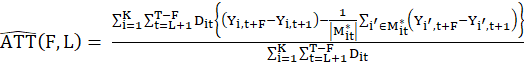

DATA AND VARIABLE DESCRIPTION
The data consists of the large set of world countries, divided into two subsets, the first containing the MPGA members and the rest are non-member countries. In order to make more transparent, objective data processing, some countries were dropped out due to data being unavailable in some domains. Before running the panel matching analysis, after filtering the primary dataset from a larger set of 174, we were able to identify 24 countries representing the treatment group, while 115 non-members were assigned to the control group (or 139 countries in total). Table 1 shows the variables used in the empirical analysis, while Table 2 shows the summary statistics of these variables. About 17,4 % of countries have joined the MPGA, while about 61,2 % signed the Kyoto Protocol promising to reduce GHG emissions in the near future. With a mean emission of 4,70 kilotonnes, CO2_pc is the most emitted gas in volume among the chosen gasses, while CH4_pc is the least emitted. The wide range in other relevant variables (gdppc, arrp, pop) indicated by the minimum and maximum levels may suggest heterogeneity of observations (countries).
| Variable | Data Source/ Description |
| https://www.fao.org/mountain-partnership/members/en22 | |
| MOUNT | Dummy variable equal 1 for the countries that are MPGA members and 0 otherwise. |
| https://ourworldindata.org23 | |
| CO2_pc | Total carbon dioxide emission per capita in levels, measured in kilotonnes. |
| CH4_pc | Total methane per capita emissions in levels (kilotonnes of CO2 equivalent). |
| N2O_pc | Total nitrous oxide per capita emissions in levels (kilotonnes of CO2 equivalent). |
| gdppc | Total GDP per capita in levels (current USD). |
| arrp | International tourism arrival per capita in levels |
| pop | This is the total population of a country. |
| https://www.chemeurope.com/en/encyclopedia/List_of_Kyoto_Protocol_signatories.html24 | |
| kyoto | Binary variable equal 1 for the countries that signed the Kyoto Protocol and 0 otherwise. |
EMPIRICAL ANALYSIS
First, we drew the plot that shows the number of matched control units that share the same treatment history as a treated observation which originates from accession to the MPGA, assigned as a treated observation in the case of four year lag. The plot given in Figure 1 shows the number of matched control units that share the same treatment history as a treated observation. We see that there are 14 treated observations for administered policy that have about 90 control units with the same treatment history when the number of lags is four. So, we have enough matched control units to test the MPGA transmitted policy along the GHG trajectories: most treated observations have more than enough matched control units.
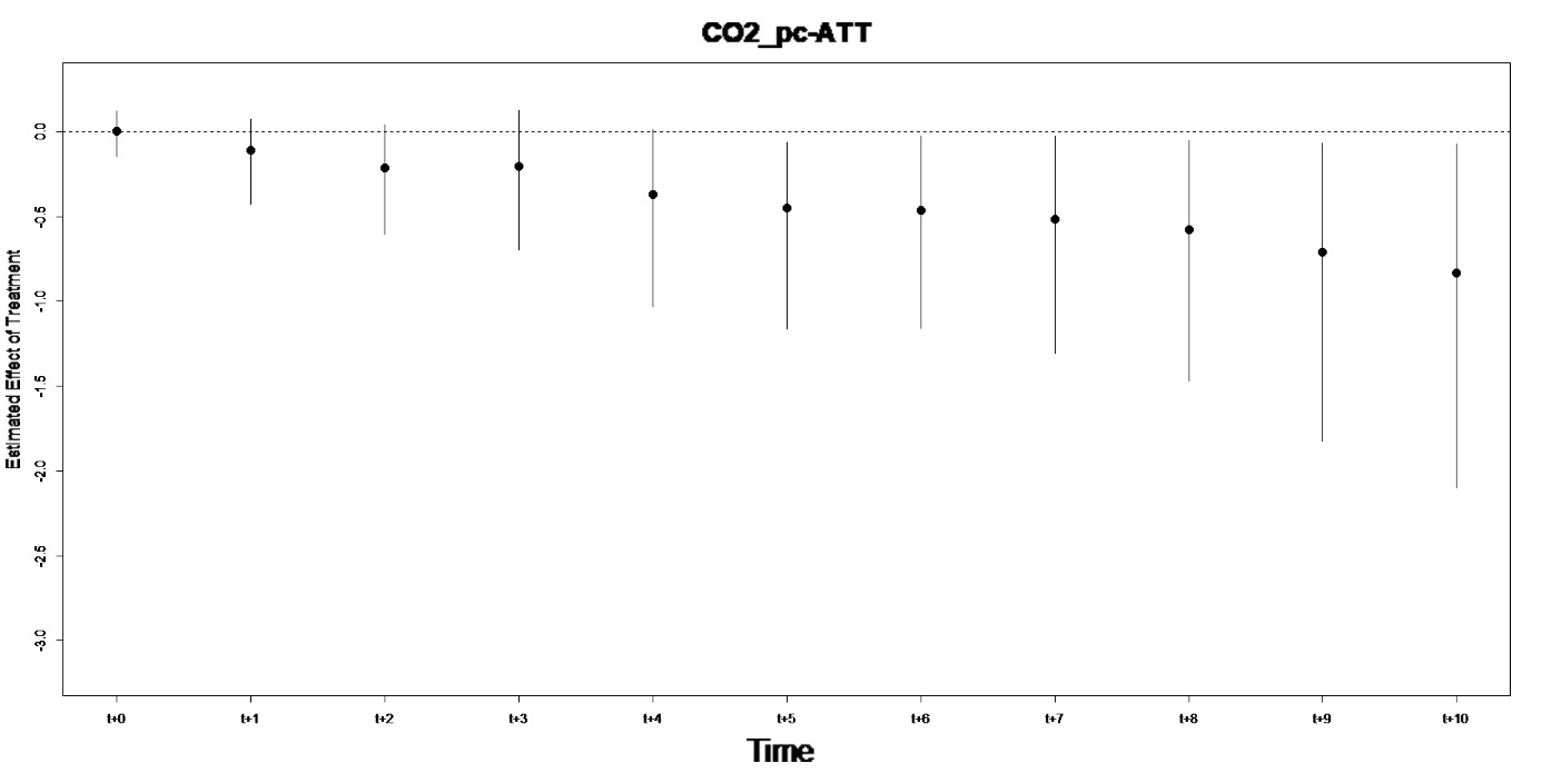
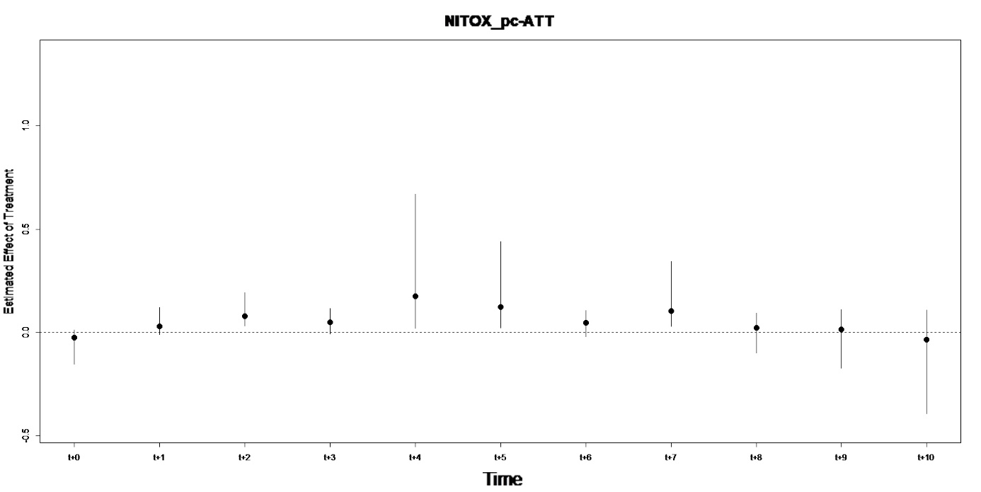
In a next step, in order to refine the matched set further, and having in mind that one of the weighting techniques had to be chosen as the best (among Mahalanobis distance matching, propensity score matching, and propensity score weighting), we proceed. So, we compare the performance of each refinement method after it had generated a new matched set. Following a result assessment, we keep the propensity score weighting refinement results as it shows to be the optimal matched set. In this auxiliary part of our panel matching research, while searching for the optimal set, all of the previously mentioned time-varying covariates were implemented e.g. indicators for economic, tourism and demographic forces, as well as a binary type of variable for the Kyoto Protocol label. The PSW refinement in our exercises essentially eliminates almost all imbalance, the standardised mean difference distance in all confounders of continuing type (yet the Kyoto covariate which is a binary type variable is somehow problematic) are minimised, e.g. has been kept to around 0. Although some degree of imbalance remains for this type of improved matching, the standardised mean difference for the lagged outcomes (CO2, CH4 and N2O, all per capita) stay rather constant over time, this is a substantial difference as before, the entire pre-treatment period. This suggests that the assumption of a parallel trend for the proposed difference-in-difference estimator is valid. This encourages us to deliberately proceed with the analysis. We now present the estimated ATTs based on the matching methods. Subsequent figures show the matching estimates of the effects of administering environmental policy which induce the act of accession to the MPGA, each for various GHG per capita types for the period of ten years after the transition point of accession to the MPGA, i.e., F = 0, 1, ..., 10. Regarding the matching set obtained by the propensity score weighting (PSW) refinement method, and when the dependent variable of interest is set up to be CO2_pc, we assessed that the point estimates of the effects for accession to the MPGA are mostly close to zero in the year of accession (see Figure2). While moving forward on a year-by-year basis, the CO2_pc variable, as an outcome, transit more and more in the intuitively expected direction. We show that in the 2nd year and future years the assumed treatment dynamics negatively impact on CO2 per capita emission. The ATT coefficient in the CO2_pc case becomes more significant and more prominently negative with the lapsing time. We report the same estimated treatment effects and confidence intervals in Table 3 (in the Appendix). It shows the estimated average treatment effect on the treated countries (ATT) when both the post-treatment (F) and pre treatment period L are set to be 10 and 4 years, respectively, along with standard error (SE) and 97,5 % confidence interval. These results suggest that the effect on CO2_pc is significant; namely, all point estimates certainly, with bootstrapped estimates, uncover negative values, after MPGA’s policy intervention. Starting from the first year, the constraints driven by policy directed to the MPGA members made substantial benefit in terms of CO2 _pc decreasing. After the turning point, which occurred in the 7th year of supposed treatment, when the average treatment effect estimate measured by CO2 emission dropped the most –by as much as 1624 kilotonnes per capita – in future years this volume in the atmosphere above treated countries changed slightly yet its volume remained always in the negative zone of values, denoting a general fall, as we had predicted. Note related to all figures 2,3 and 4: The average treatment effects are represented by point estimates over time (in years), with lines corresponding to standard errors obtained with 1000 bootstrap iterations. Here 2,5 % and 97,5 % are quantiles of the bootstrapped estimates reported. Propensity score weighting was used to create the matched sets. The Figure 3 shows the level of CH4_pc movement in the MPGA group after acceptance of mandatory environmental policy. The methane emissions per capita (CH4_pc), at first paradoxically increased following the implementation of environment-led protection policy covered by appropriate laws, but the difference was insignificant. The results indicate an expected decrease of methane per capita, as expected after the adoption of environmental policy, in the years after the second year. Yet, the bootstrapped estimates yield both positive and negative values in the entire interval, suggesting little evidence of a non-zero effect. Summarising the case of the CH4_pc trajectory path on the change due to MPGA association, we show that the effect sizes had a strange trajectory path, zigzagging negatively but were insignificant. Furthermore, in the 5th year, beside others, we underline that the causal impact became borderline significant. The fall in the emission of CH4_pc in that year, we assess to be about 0,177 kilotonnes. According to Figure 4 we cannot find sufficient evidence for our hypothesis that MPGA induced environmental policy would reduce N2O_pc emission in the treatment group of countries. Some of the treatment effect estimates are positive, more precisely in the years: four, five and seven) indicating that an assumed environmental law regulation coming into force causally increases emission of N2O_pc. The weak magnitude in the second year brought in effect the significant impacts. We also noticed positive impacts paradoxically unevenly scattered which are not otherwise negligible in the other observed years. In some of them their confidence intervals were zero.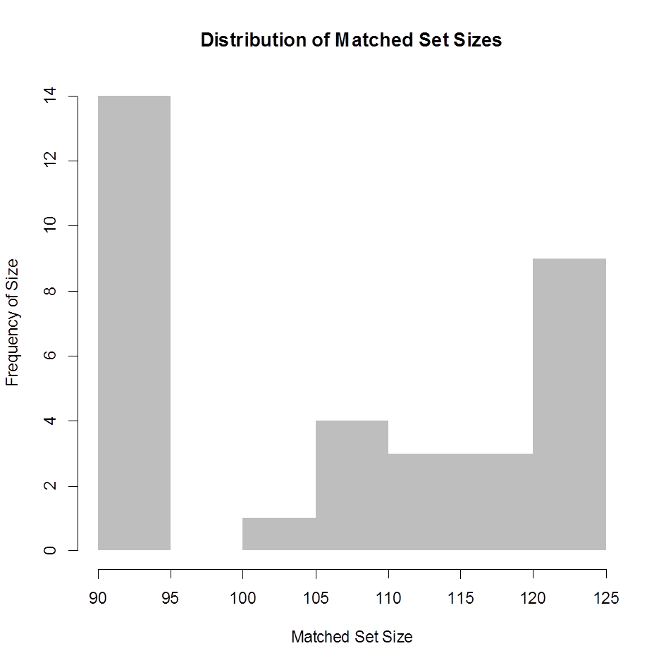
CONCLUSIONS
This study was designed to determine whether the interventions to reduce GHG emissions under the MPGA significantly reduced the countries’ carbon footprint, or whether they report more negative outcomes than the control group of countries. We can, without hesitation, report, and this is the most important conclusion, that: the mountainous countries, while taking care to environmental sustainability, given an incentive to invest in carbon abatement become lower emitters, on per capita basis, of carbon dioxide greenhouse gas after accession to the MPGA. Countries that made interventions to reduce GHG emissions after joining the MPGA were also found to have lower levels of small particles linked to methane per capita but only at borderline significance level. We also found counter-intuitive evidence that intervention based on a commitment to community efforts regarding environmental sustainability, recorded in the MPGA database, contributed to an increase in nitrous oxide emissions per capita in a few years following the intervention. Results that link carbon dioxide and methane may enhance, we hope, the domestic-level policies introduced by governmental authorities in future. This will curb environmental vulnerability around a typical MPGA country more effectively. In response to the N2O per capita environmental indicator spread, despite intervention, a mission to improve environmental care throughout the mountain world, will not suffice. We recognise, as a self-criticism that our research objectives would not have been met if the panel matching estimation strategy suffered from bias of any sort, such as if the pivotal variable of instrument intervention is not fairly selected. We had focused on only one option of joining MPGA, at governmental level. Yet this kind of connections occasionally overlapped with different kinds of accessions to MPGA within the same time period, for example at intergovernmental or regional levels. Without more data, especially a richer specification of covariates, we also risk misspecification bias of some sort. We had unfortunately focused only on economic, touristic, demographic and institutional habitus of covariates that linked the commitment of nations to reduce GHG emissions, and which subsequently made the treatment subsample. Those inferences that had been extracted from the designed DiD-PM method, we hope modelled GHG complexities, giving the most plausible outputs. Yet we believe the estimated null results, keeping those limitations in mind, are worth reporting given the widespread and long-term impact of MPGA policies on humanity. Especially, we may say concluding our narrative if the vicious cycle expressed in the growing population that transmits perpetual economic and tourism growth fosters the endless increase in carbon footprint. In spite of these limitations, we believe this estimation strategy of ours provides the most robust assessment of the effects of MPGA policies on environmental indicators spread to date, having in mind that we have long ago surpassed the peak of GHG saturation globally. We hope others will be able to build upon our results to further assess the relevance, benefits and feasibility of various policy measures undertaken by MPGA regarding the global growth in the carbon footprint.