1. Introduction
The term loxodrome comes from the Greek loxos (λοξός): slanting + dromos (δρόμος): road. In English, loxodrome and rhumb line are synonyms. The word rhumb probably comes from the Spanish/Portuguese rumbo/rumo (course, direction), Greek rombos (ρόμβος) or Latin rhombus: tern (Simović 1978,Lapaine 1993,Viher i Lapaine 1998,Lapaine 2006).
The first scientist who introduced the term loxodrome was Pedro Nunes (lat. Petrus Nonius, Alcácer do Sal, 1502 – Coimbra, 11 August 1578), a Portuguese mathematician, cosmographer and professor. He is considered one of the greatest mathematicians of his time. He is best known for his contributions to the navigation technique, which was extremely important at the time of the discovery of new territories. He is the inventor of several measuring devices, including the vernier (nonius), named after his Latin surname. Nunes was the first to understand why a ship that sails in a constant direction will not sail along the geodetic line, i.e. the shortest path connecting two points on Earth, but on a spiral course called a loxodrome. In the work Tratado em defensam da carta de marear (Treatise on the Defense of Maritime Charts) he advocated showing parallels and meridians as straight lines on navigational charts. However, he wasn't sure how to solve the problem. This question remained unsolved until Gerhard Mercator discovered a projection that is still used today and is called the Mercator projection after him (Simović 1978,Lapaine 1993,Viher i Lapaine 1998,Lapaine 2006).
Alexander (2004) mainly deals with the historical development and connection of the loxodrome with the Mercator projection.Petrović (2007) considers the loxodrome on the rotational ellipsoid, but only gives equations without a more detailed derivation and without concrete applications.
This article describes the results of the authors' research, which is based on Lapaine's 1993 article and is an extension of it. First, a loxodrome is defined on an arbitrary surface, and then it is specified on a sphere and on a rotational ellipsoid. It is shown that by analogy with the loxodrome on the sphere, the loxodrome on the ellipsoid can also be treated, only the formulas are more complex. In addition, the first and second geodesic problems for the loxodrome on the sphere and on the rotating ellipsoid are solved.
Let Ω be the area in the plane, and let
be the mapping of the area Ω into the three-dimensional space R3. Let us mark:
By mapping
, a surface in space is defined. There, some other conditions are usually imposed on the mapping
, for example, that the mapping is bijective, continuous, differentiable up to some order, etc. By definition, u-lines are curves for which v = const., while v-lines are curves for which u = const.
A straight line in a rectangular Cartesian system (u,v) has the well-known property that it closes equal angles with all u--lines (v-lines). The question naturally arises: is there such a curve on the surface that closes equal angles with all u--lines (v-lines)? If it exists, such a curve is called a loxodrome.
2. Definition and Equation of Loxodrome
Let
be the differential of the mapping
It can be written
Then it is
i.e. the first differential form of the mapping
is:
where we marked as usual in mathematics:
It is possible to interpret the first differential form as a cosine low for the triangle described by the relation
Let
denote the tangent vector to any curve, and
the tangent vector to the u-curve at the observed point. Assume
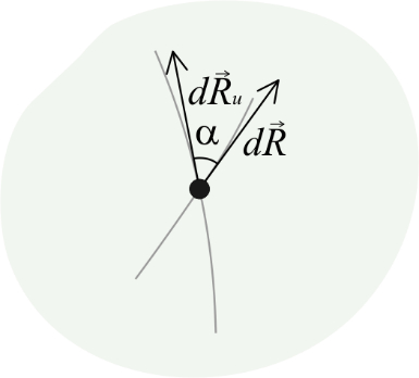
Let us denote by α the angle between the curve and the u-curve and remember how this angle can be determined (Figure 1).
Figure 1. Vectors dR, dRu at some point on the surface and angle α is the angle between some curve and u-curve / Slika 1. Vektori dR, dRu u nekoj točki na plohi i kut α kut između neke krivulje i u-krivulje
The scalar product of vectors
and
is
where:
From there follows
because we assumed
and
This expression is valid for any curve on the surface. Furthermore, according to the basic trigonometric relation sin2α + cos2α=1 we have:
and from there
Let us conclude that the following formulas are valid for any curve on the surface parametrized by the parameters u and v:
Definition. Let α = const. If there is a solution of the differential equation (3), (4) or (5) in addition to (2), it is called a loxodrome on the surface defined by (1).
We leave the solving of this general task to those interested, and below we will solve simpler cases important for cartography and geodesy. Let us also note that equations (2)–(5) are not mutually independent. For example squaring and adding equations (3) and (4) yields (2), and dividing (4) and (3) yields (5).
3. The equation of the curve on the surface where u-lines and v-lines form an orthogonal network
Let us take the special case of a surface for which
i.e. let the u-curves and v-curves intersect at right angles. Expressions (2)–(5), which are valid for any curve on the surface, for the surface for which F = 0 read like this (right triangle, theorem of Pythagora):
If still α = const. then (7), (8) and (9) along with (6) are the differential equations of the loxodrome in three different forms. We will consider the special cases α =kπ, k∈Z and α=k π/2, k∈Z in section 7.
4. The Equation of the Loxodrome on the Sphere
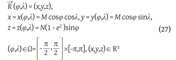
Since in geodesy and cartography parameters are usually not denoted by u and v, but by φand λ, instead of u and v in the following part of the paper we will use φand λ. Let us recall that for R = const. The mapping
defines a sphere with its center at the origin of the coordinate system and radius R.
The coefficients of the first differential form of this mapping are:
E=R2, F=0, G=R2cos2φ.
Accordingly, the differential expressions (6)–(9) for any curve on the sphere are:
Let us agree that the angle α will have a value from the interval (0,2π). It is the azimuth that will be measured clockwise so that the relationships shown inTable 1 apply.
Table 1. Basic relationships between latitude, longitude and azimuth / Tablica 1. Osnovni odnosi između geografske širine, geografske dužine i azimuta
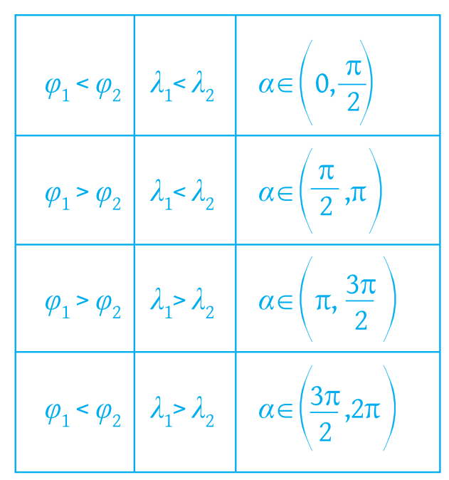
If we accept the relations fromtable 1., and the fact that the length of the arc from the curve must be positive, then in formulas (12) and (13) it is sufficient to take only the positive sign.
Let α = const. The differential equation of the loxodrome on the sphere is then e.g. (11), and can be solved in the following simple way:
cos α ∫ ds = R ∫ dφ,
which after integration gives
namely the loxodrome equation that connects the latitude φ and the arc length s. That loxodrome passes through a point with latitude φ1 and at that point the arc length is 0.
Loxodromes on a sphere are generally spiral curves that wrap around each pole an infinite number of times (Figures 4 and5), and as we shall soon see, never reach it, although their length is finite.
The length of the loxodrome from pole to pole is equal to the length of the arc of the meridian divided by the cosine of the angle α. Indeed, in formula (14) we should put φ1=-π/2, s1=0, φ=π/2, so we obtain s=Rπ\cosα, α≠π/2+kπ, k∈Z.
If we start with the differential equation (12), we cannot integrate it immediately, but first we should express φ by means of λ or s. Therefore, we prefer to take equation (13), which can be integrated if we write it in the form
After integration we get
If we want the loxodrome to pass through the point with geographical coordinates (φ1, λ1), it is necessary to take the integration constant β
Finally, if we want the relationship between λ and s we can write
If s = 0, then λ = λ1.
Figure 2. Loxodrome on a sphere / Slika 2. Loksodroma na sferi
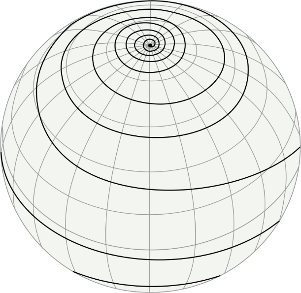
Figure 3. Loxodrome in the stereographic projection of the northern hemisphere / Slika 3. Loksodroma u stereografskoj projekciji sjeverne polusfere
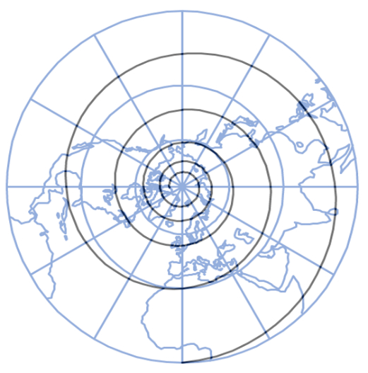
Figure 3 shows part of the loxodrome in the northern hemisphere in the stereographic projection. The equation of that loxodrome in the polar coordinate system in the plane of the stereographic projection is:
In mathematics, such a curve is called a logarithmic spiral.
5. Isometric Latitude and Loxodrome
The isometric latitude q on the sphere in the theory of map projections is defined by the geographic latitude φ and the differential equation
The solution of differential equation (18) is
with the assumption that for the integration constant we took the value that gives φ = 0 for q = 0. The inverse equation is:
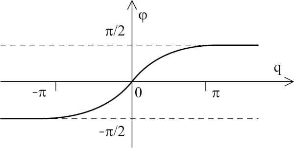
A graphic representation of the mutual dependence of geographic and isometric latitude is given inFigure 4.
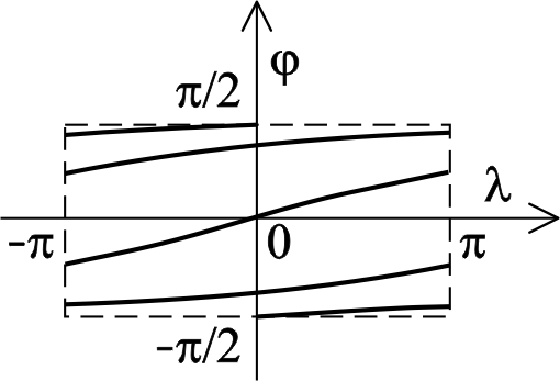
Figure 4. Relationship between geographic and isometric latitude. The geographic latitude φ ∈ (-π/2,π/2) corresponds to the isometric q ∈( -∞,∞) and vice versa, formulas (19) and (20). / Slika 4. Odnos između geografske i izometrijske širine. Geografskoj širini φ ∈ (-π/2,π/2), odgovara izometrijska širina q ∈( -∞,∞) i obratno, formule (19) i (20).
These relations are easily derived from the definition of isometric latitude
Furthermore, the differential equation (15) written by using the isometric latitude q becomes very simple and reads
After integration, we get the equation of the loxodrome on the sphere in the form
where β is the integration constant. If we want the rhombus to pass through the point with coordinates (q1λ1), it is necessary to take the integration constant β
6. Generalized Longitude λ
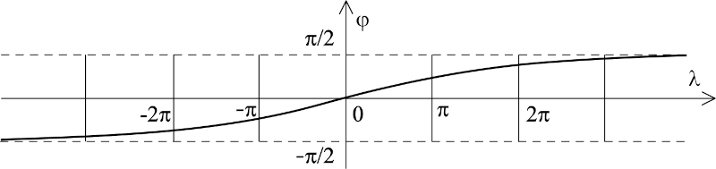
We notice that for any φ ∈ (-π/2,π/2), λ determined according to (16) is a real number that generally does not have to be from the interval (-π,π) and does not have the meaning of longitude in the usual sense (Figure 5). This is also clearly seen when determining λ by formula (23).
Figure 5. Loxodrome in the coordinate system λ,φ, where λ is longitude in the broad sense, and β = 0. / Slika 5. Loksodroma u koordinatnom sustavu λ,φ, gdje je λ geografska dužina u širem smislu, a β = 0.
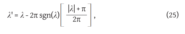
That is why λ determined by relation (15) or (23) is called longitude in a broader sense. The corresponding value of longitude λ' from the interval (-π,π) will be obtained as a remainder when dividing by 2π, i.e. by applying the formula
where sgn(λ) is equal to 1, 0 or –1, but according to whether λ is greater than, equal to or less than zero, and the square brackets indicate the largest integer function, i.e. [x] is the largest integer that is less than x or equal to x (Figure 6).
Figure 6. Loxodrome in the coordinate system λ, φ , where λ is the longitude in the usual sense / Slika 6. Loksodroma u koordinatnom sustavu λ, φ, gdje je λ geografska dužina u uobičajenom smislu
If λ ∈ (-π,π), then the longitude in a broader sense coincides with the usual longitude.
Numerical example 1
Given:
φ1 = 0°, λ1 = 0°
φ1 = 45°
α = 45°
Looking for: λ2
Calculated:
Using expression (19), we calculate
q1=0, q2=0,88137, β=0, λ2=q2,
so by applying the formula (23), the value of longitude λ2 in the broader sense in radians is 0.88137, i.e. in degrees 50°29'56''. As the calculated value is within the interval (-π,π), the longitude coincides with the common longitude.
Numerical example 2
Given:
φ1 = 0°, λ1 = 0°
φ1 = 45°
α = 80°
Looking for: λ2
Calculated:
Using expression (19), we calculate
q1=0, q2=0,88137, β=0, λ2=q2tan 80°=4,998518.
By applying expression (23), the value of geographic longitude in the broader sense is calculated, which in radians is 4.99852, that is, in degrees 286°23'38''. Since the calculated value is not within the interval (-π,π), the geographic longitude in the usual sense can be calculated using formula (25), which amounts to –1.28467 in radians, or –73°36'22'' in degrees.
7. Special Cases
Meridians and parallels are special cases of loxodrome. For meridians α =kπ, k∈Z, Z is the set of all integers, and for parallels α=π/2+kπ, k∈Z- Indeed, if we take α =kπ, k∈Z, then (14) turns into s=R(φ-φ1), and (15) into λ = λ1.
For α=π/2+kπ, k∈Z, (14) becomes φ = φ1, and the differential equation ds=R cos φ1 dλ gives the solution s=R cos φ1 (λ-λ1).
8. Definition of Isometric Latitude Using Geographic Longitude
It is well known that latitude and longitude can also be defined using the corresponding angles related to the Earth's sphere or globe. Thus, latitude is the angle that the normal of the observed point closes with the equatorial plane. Longitude is the angle between the meridian passing through the observed point and the prime meridian. The question arises whether the isometric latitude can be interpreted in a similar way.Heck (1987) says in his famous monograph: "While the latitude φ can be given a geometric meaning of the direction of the normal on the surface, the numerical values of the isometric latitude cannot be interpret visually." We will show that it is not so, but that the isometric latitude can be interpret visually.
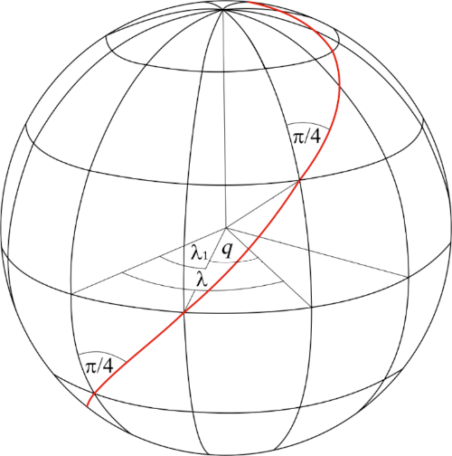
For this purpose, through any point with coordinates (φ,λ)∈ (-π/2,π/2) × (-π,π) we draw a loxodrome on the sphere at an angle α=π/4 (Figure 7).
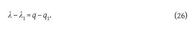
The loxodrome equation according to (23) and (24) then reads
One nice property of such a loxodrome can be read from there: the difference in the isometric latitude of any two points on the loxodrome that closes the angle α=π/4 on the sphere with meridians is equal to the difference in the geographic longitudes of those points. Geographical longitudes are understood in a broader sense.
The following is valid for the point where the loxodrome crosses the equator
φ1=q1=0.
Now (23) can be written in the form
q=λ-λ1,
which enables this definition of isometric latitude:
Definition. The isometric latitude of any point on the sphere is equal to the difference between the longitude (in a broader sense) of that point and the longitude of the point where the loxodrome drawn through the observed point at an α=π/4 to the meridians (parallels) intersects the equator (Figure 7).
Figure 7. Isometric latitude q as the difference of geographic longitudes / Slika 7. Izometrijska širina q kao razlika geografskih dužina
So, although isometric latitude contains the word "latitude" in its name and is usually formally defined using geographic latitude, it has just been explained how it can be very simply displayed and interpreted on a sphere as the difference of two longitudes. Analogous considerations apply to the loxodrome on the rotating ellipsoid.
9. Basic Tasks Along the Loxodrome on the Sphere
The first geodesic task for the loxodrome on a sphere of given radius R.
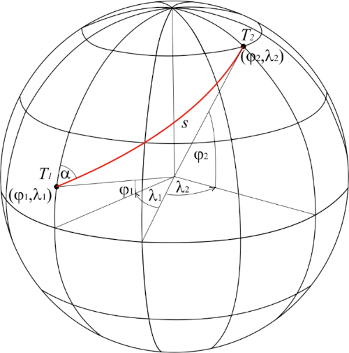
Point T1 (φ1,λ1) is given, the loxodrome that passes through that point closes the angle α to the meridians and the length of the arc is s. We are looking for point T2 (φ2,λ2) on that loxodrome, which is distant from point T1 along the loxodrome by s.
Solution
According to expression (14) we have
Then according to (19) we calculate
According to (23) we have
λ1=q1 tanα+β, λ2=q2 tanα+β,
and from there
λ2=(q2-q1) tanα+λ1.
Figure 8. With the first and second geodesic tasks for the loxodrome on the sphere / Slika 8. Uz prvi i drugi geodetski zadatak za loksodromu na sferi
Numerical example
Given:
Point T1 (Zagreb): φ1 = 46° N, λ1 = 16° E
α = 158°
s = 420 000 m
R = 6 370 000 m
Looking for: φ2 i λ2
Calculated:
Point T2 (Dubrovnik): φ2= 42°30' N, φ2 = 18° E
The second geodetic problem for the loxodrome on a sphere of given radius R
The points T1 (φ1,λ1) and T2 (φ2,λ2) are given on the sphere of radius R. The angle to the meridians enclosed by the loxodrome connecting these two points is sought, and the length of the arc s of the loxodrome between these two points.
Solution:
First, we calculate according to (19).
Then according to (23) we have
λ1=q1 tan α+β, λ2=q2 tan α+β
And from there
Finally, according to (14)
Numerical example:
Given:
Point T1 (Zagreb): φ1 = 46° N, λ1= 16° E
Point T2 (Dubrovnik): φ2 = 42°30' N, λ2= 18° E
R = 6 370 000 m
Looking for: α and s
Computed:
α = –22°15'03"+k·180°
Since φ1>φ1 and λ1<λ1 according totable 1 we choose that α for which α ∈ (π/2, π). Therefore, α = 157°44'56". After that, we get s = 420 km.
RemarkThe question arises: how many loxodromes are there that connect the two points T1 and T2 on the sphere? The answer is: infinitely many, we just have to remember that instead of longitude (e.g. λ2) it is possible to use longitude in the broader sense λ2 + 2kπ, k∈Z.
Numerical example
If the starting point T1 is Zagreb with coordinates φ1 = 46° and λ1 = 16°, and the end point T2 is Dubrovnik with coordinates φ2 = 42°30', λ2 = 18° + k 360° then for:
k = 0, λ2 = 18° calculated azimuth α = 157°44'56", distance s = 420 km
k = 1, λ2 = 378° calculated azimuth α = 90°46'25'', distance s = 28 818 km
k = 2, λ2 = 738° calculated azimuth α = 90°23'17'', distance s = 57 473 km
k = 3, λ2= 1098° calculated azimuth α = 90°15'32'', distance s = 86 129 km
etc
10. Loxodrome on a rotational ellipsoid
The following expressions define in geodesy and cartography a rotational ellipsoid with the center at the origin of the coordinate system, the semi-major axis a and the numerical eccentricity e:
We marked
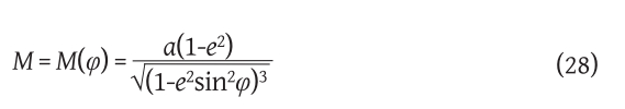
radius of curvature of the meridian and
radius of curvature of the intersection along the first vertical. The coefficients of the first differential form of this mapping are:
E = M2, F=0, G=N2cos2φ
Accordingly, the differential expressions (6)–(9), with agreement on the sign of the azimuth α according toTable 1, for any curve on the rotational ellipsoid are:
Let α = const. The differential equation of the loxodrome on the rotating ellipsoid is then e.g. (31), and can be solved as follows:
cosα ∫ds=∫ Mdφ,
which after integration gives
where
so (34) is the equation of the loxodrome connecting the latitude φ and the arc length s. This loxodrome passes through a point with latitude φ1 and at that point the arc length is 0.
Unlike the derivation of the loxodrome equation on the sphere, the integral on the right in (35) is an elliptic integral that appears when calculating the length of the arc of the meridian on the rotational ellipsoid, and which cannot be directly integrated, but instead, series or some other mathematical methods are applied. Lapaine (1990, 1994) showed that for calculating the length of the arc of the meridian from the equator to the geodetic latitude φ, a suitable formula is the following
where A, c1, c2, …, c5 are the corresponding coefficients.
In formula (36), the length of the arc of the loxodrome is expressed as a function of geodetic latitude. If it is necessary to express the geodetic latitude as a function of the length of the arc of the loxodrome, then we can use the formula that determines the geodetic latitude of a point on the meridian for which the length of the arc of the meridian from the equator to that point is known Lapaine (1990, 1994):
where c1, c2, …, c5 are corresponding coefficients, and
Loxodromes on a rotational ellipsoid, like on a sphere, are generally spiral curves that wrap around each pole an infinite number of times, and never reach it, although their length is finite. The length of the loxodrome from pole to pole is equal to the length of the arc of the meridian divided by the cosine of the angle α.
Indeed, in formula (34) we should put φ1=π/2, φ=π/2, so we get
If we start with the differential equation (32) we cannot integrate it immediately, but we should first express φ by means of λ or s. Therefore, we prefer to take equation (33) which can be integrated if we write it in the form
After integration we get
If we want the loxodrome to pass through the point with geodetic coordinates (φ1, λ1), it is necessary to take the integration constant β
Finally, if we want a connection between the longitude λ and the arc length of the loxodrome s, it is necessary to include φ from (40) including (41), (42) and (43) in (45).
11. Isometric Latitude and Loxodrome on a Rotational Ellipsoid
Taught by the experience from the previous sectionis on isometric latitude and loxodromes on a sphere, let us try an analogous approach on a rotational ellipsoid. The isometric latitude q in the theory of map projections is defined by means of the geodetic latitude φ and the differential equation
The solution of differential equation (47) is
with the assumption that for the integration constant we took the value that gives φ = 0 for q = 0. The inverse function cannot be written in a finite form using elementary functions, but different approximation procedures or approximate formulas are used (Frančula 2004).
If the conformal latitude χ is introduced as follows
then between it and the isometric latitude q, analogous to relations (21), the following relations apply:
Furthermore, the differential equation (44) written with the help of the isometric latitude q becomes very simple and formally reads as in (22), it is only necessary to note that here we are talking about the isometric latitude q on the rotational ellipsoid defined by (48). After integration, we get the equation of the loxodrome on the rotational ellipsoid in the form (23). If we want the rhombus to pass through the point with geographic coordinates(q1, λ1), it is necessary to take the integration constant β as in (24).
12. Basic Tasks Along the Loxodrome on the Rotational Ellipsoid
The first geodesic problem for a loxodrome on a rotational ellipsoidThe point T1 (φ1,λ1) on the rotational ellipsoid with semi-axes a and b is given, the loxodrome that passes through that point closes the angle α to the meridians and the length of the arc is s. The point T2 (φ2,λ2) is sought on that loxodrome which is far from the point T1 along the loxodrome for s.
Solution:
According to formula (34) we can write
sm (φ2) = s cos α + sm (φ1).
Then according to formulas (40)-(42) we calculate φ2=φ2(ψ), where
Now, according to formula (48) we can calculate
q1 = tanh(-1)(sinφ1)-e tanh(-1)(e sinφ1),
q2 = tanh(-1)(sinφ2)-e tanh(-1)(e sinφ2),
and finally based on formulas (45) and (46)
λ2=(q2-q1) tanα + λ1.
The second geodesic problem for a loxodrome on a rotational ellipsoidPoints T1 (φ1,λ1) and T2 (φ2,λ2) are given on the rotational ellipsoid with semi-axes a and b. The angle α to the meridians enclosed by the loxodrome connecting these two points is sought, and the length s of the arc from the loxodrome between these two points.
Solution
First, we calculate using formula (48)
q1 = tanh(-1)(sinφ1)-e tanh(-1)(e sinφ1),
q2 = tanh(-1)(sinφ2)-e tanh(-1)(e sinφ2).
Then we have
and finally
13. Conclusion
In this paper, the close connection between isometric latitude and loxodrome is explained in detail. A new generalized definition of the loxodrome on any surface is proposed. Its differential equations are derived, which are solved on a sphere and on a rotational ellipsoid. A new concept of generalized geographic longitude was introduced, which appears in a natural way when solving the differential equation of the loxodrome. Generalized longitude allows defining isometric latitude in a new way. The relations between the isometric latitude and the geographic longitude on the sphere and geodetic longitude on the ellipsoid, are derived. At the end, basic geodesic tasks are solved along the loxodrome on the sphere and on the rotational ellipsoid.
1. Uvod
Riječ loksodroma dolazi od grčkoga loxos (λοξός): koso + dromos (δρόμος): put. Na engleskom jeziku susreću se kao sinonimi loxodrome i rhumb line. Riječ rhumb vjerojatno dolazi od španjolskoga/portugalskoga rumbo/rumo (kurs, smjer), grčkoga rombos (ρόμβος) ili latinskoga rhombus: čigra, zvrk (Simović 1978,Lapaine 1993,Viher i Lapaine 1998,Lapaine 2006).
Prvi znanstvenik koji je uveo pojam loksodrome bio je Pedro Nunes (lat. Petrus Nonius, Alcácer do Sal, 1502 – Coimbra, 11. 8. 1578), portugalski matematičar, kozmograf i profesor. Smatra se jednim od najvećih matematičara svojega doba. Najpoznatiji je po doprinosima u tehnici navigacije, što je bilo iznimno važno u to doba otkrića novih teritorija. Izumitelj je nekoliko mjernih sprava, među kojima je i nonius, nazvan prema njegovu latinskom prezimenu. Nunes je prvi shvatio zašto brod koji plovi stalnim smjerom neće ploviti uzduž geodetske linije, tj. najkraćeg puta koji spaja dvije točke na Zemlji, nego po spiralnom kursu koji se naziva loksodroma. U djelu Tratado em defensam da carta de marear (Rasprava o obrani pomorskih karata) zalagao se za prikazivanje paralela i meridijana u obliku ravnih crta na navigacijskim kartama. Međutim, nije bio siguran kako riješiti taj problem. To je pitanje ostalo neriješeno sve dok Gerhard Mercator nije otkrio projekciju koja se i danas upotrebljava i koja se po njemu naziva Mercatorovom projekcijom (Simović 1978,Lapaine 1993,Viher i Lapaine 1998,Lapaine 2006).
Alexander (2004) se pretežno bavi povijesnim razvojem i vezom loksodrome s Mercatorovom projekcijom.Petrović (2007) razmatra loksodromu na rotacijskom elipsoidu, ali daje samo jednadžbe bez detaljnijeg izvoda i bez konkretnih primjena.
Ovaj članak opisuje rezultate istraživanja autora koja se temelje na Lapaineovu članku iz 1993. godine i predstavljaju njegovu nadogradnju. Najprije se definira loksodroma na proizvoljnoj plohi, a zatim konkretizira na sferi i na rotacijskom elipsoidu. Pokazuje se da se po analogiji s loksodromom na sferi, može tretirati i loksodroma na elipsoidu, samo što su formule složenije. Osim toga, rješavaju se prvi i drugi geodetski zadatak za loksodromu na sferi i na rotacijskom elipsoidu.
Neka je Ω područje u ravnini, a
preslikavanje područja Ω trodimenzionalan prostor R3. Označimo:
Preslikavanjem
definirana je ploha u prostoru. Tu se obično zadaju još neki uvjeti na preslikavanje
, npr. da je to preslikavanje bijektivno, neprekidno, diferencijabilno do nekog reda itd. Po definiciji u-linije su takve krivulje za koje je v=const., dok su v-linije takve krivulje za koje je u=const.
Pravac u ravnini u pravokutnom kartezijevom sustavu (u,v) ima poznato svojstvo da sa svim u-linijama (v-linijama) zatvara jednake kutove. Prirodno se postavlja pitanje: postoji li na plohi takva krivulja koja sa svim u-linijama (v-linijama) zatvara jednake kutove? Ako postoji, takva se krivulja naziva loksodromom.
2. Definicija i jednadžba loksodrome
Neka je
diferencijal preslikavanja
Može se napisati
Tada je
tj. prva diferencijalna forma preslikavanja
je:
gdje smo označili kao što je uobičajeno u matematici:
Moguća je interpretacija prve diferencijalne forme kao kosinusnog poučka za trokut koji opisuje relacija
Označimo s
vektor tangente na bilo koju krivulju, a
vektor tangente na u-krivulju u promatranoj točki. Pretpostavimo
Označimo s α kut između krivulje i u-krivulje i podsjetimo se kako se taj kut može odrediti (slika 1).
Skalarni produkt vektora
i
je
gdje su:
Odatle slijedi
jer smo pretpostavili
i zatim
Taj izraz vrijedi za bilo koju krivulju na plohi. Nadalje, prema osnovnoj trigonometrijskoj relaciji sin2α + cos2α=1 imamo:
i odatle
Zaključimo da sljedeće formule vrijede za bilo koju krivulju na plohi parametriziranoj parametrima u i v:
Definicija. Neka je α = const. Ako postoji rješenje diferencijalne jednadžbe (3), (4) ili (5) uz (2), ono se zove loksodroma na plohi definiranoj s (1).
Rješavanje tog općenitog zadatka prepuštamo zainteresiranima, a mi ćemo u nastavku riješiti jednostavnije slučajeve važne za kartografiju i geodeziju. Uočimo još da jednadžbe (2)–(5) nisu međusobno nezavisne. Npr. kvadriranjem i zbrajanjem jednadžbi (3) i (4) dobije se (2), a dijeljenjem (4) i (3) dobije se (5).
3. Jednadžba krivulje na plohi na kojoj u-linije i v-linije čine ortogonalnu mrežu
Uzmimo poseban slučaj plohe za koju vrijedi
tj. neka se u-krivulje i v-krivulje sijeku pod pravim kutom. Izrazi (2)–(5), koji vrijede za bilo koju krivulju na plohi, za plohu za koju je F = 0 glase ovako (pravokutan trokut, Pitagorin poučak):
Ako je još α = const., tada su (7), (8) i (9) uz (6) diferencijalne jednadžbe loksodrome u tri različita oblika. Posebne slučajeve α =kπ, k∈Z and α=k π/2, k∈Z razmatrat ćemo u poglavlju 7.
4. Jednadžba loksodrome na sferi
Budući da se u geodeziji i kartografiji parametri obično ne označavaju s u i v, nego s φ i λ, umjesto u i v u tekstu koji slijedi upotrebljavat ćemo φ i λ. Prisjetimo se da se za R = const. Preslikavanjem
definira sfera sa središtem u ishodištu koordinatnog sustava i polumjerom R.
Koeficijenti prve diferencijalne forme toga preslikavanja su:
E=R2, F=0, G=R2cos2φ.
Prema tome diferencijalni izrazi (6)–(9) za bilo koju krivulju na sferi su:
Dogovorimo se da će kut α imati vrijednost iz intervala (0,2π). To je azimut koji će se mjeriti u smjeru kazaljke na satu tako da vrijede odnosi prikazani utablici 1.
Prihvatimo li odnose iztablice 1, te činjenicu da duljina luka s krivulje mora biti pozitivna, tada je u formulama (12) i (13) dovoljno uzeti samo pozitivan predznak.
Neka je α = const. Diferencijalna jednadžba loksodrome na sferi je tada npr. (11), a može se riješiti na sljedeći jednostavan način:
cos α ∫ ds = R ∫ dφ,
što nakon integracije daje
i to jednadžba loksodrome koja povezuje geografsku širinu φ i duljinu luka s. Ta loksodroma prolazi točkom s geografskom širinom φ1 i u toj je točki duljina luka 0.
Loksodrome na sferi su općenito spiralne krivulje koje se omataju oko svakog pola beskonačno mnogo puta (slike 4 i5), i kao što ćemo uskoro vidjeti, do njega nikad ne stižu, premda je njihova duljina konačna. Duljina loksodrome od pola do pola jednaka je duljini luka meridijana podijeljenog kosinusom kuta α. Zaista, u formulu (14) treba staviti φ1=-π/2, s1=0, φ=π/2, pa se dobije s=Rπ\cosα, α≠π/2+kπ, k∈Z.
Ako krenemo s diferencijalnom jednadžbom (12) ne možemo je odmah integrirati, nego bi najprije trebalo izraziti φ s pomoću λ ili s. Stoga ćemo radije uzeti jednadžbu (13) koja se može integrirati ako je napišemo u obliku
Nakon integriranja dobijemo
Ako želimo da loksodroma prolazi točkom s geografskim koordinatama (φ1,λ1), potrebno je za integracijsku konstantu β uzeti
Konačno, ako želimo vezu između λ i s možemo napisati
Ako je s = 0, onda je λ = λ1.
Naslici 3 prikazan je dio loksodrome na sjevernoj polusferi u stereografskoj projekciji. Jednadžba te loksodrome u polarnom koordinatnom sustavu u ravnini stereografske projekcije glasi
U matematici se takva krivulja naziva logaritamskom spiralom.
5. Izometrijska širina i loksodroma
Izometrijsku širinu q na sferi u teoriji kartografskih projekcija definiramo s pomoću geografske širine φ i diferencijalne jednadžbe
Rješenje diferencijalne jednaždbe (18) je
uz pretpostavku da smo za integracijsku konstantu uzeli onu vrijednost koja za φ = 0 daje q = 0. Obratna veza je:
Grafički prikaz međusobne ovisnosti geografske i izometrijske širine dan je naslici 4.
Iz definicije izometrijske širine lako se izvedu ove relacije
Nadalje, diferencijalna jednadžba (15) napisana uz pomoć izometrijske širine q postaje vrlo jednostavna i glasi
Nakon integriranja dobijemo jednadžbu loksodrome na sferi u obliku
gdje je β konstanta integracije. Ako želimo da loksodroma prolazi točkom s koordinatama (q1λ1), potrebno je za integracijsku konstantu β uzeti
6. Poopćena geografska dužina λ
Uočimo da je za bilo koji φ ∈ (-π/2,π/2), λ određen prema (16) realan broj koji općenito ne mora biti iz intervala (-π,π) te nema značenje geografske dužine u uobičajenom smislu (slika 5). To se također jasno vidi pri određivanju λ po formuli (23).
Zbog toga λ određen relacijom (15) ili (23) zovemo geografskom dužinom u širem smislu. Odgovarajuća vrijednost geografske dužine λ' iz intervala (-π,π) dobit će se kao ostatak pri dijeljenju s 2π, odnosno primjenom formule
gdje je sgn(λ) jednako 1, 0 ili –1, već prema tome je li λ veće, jednako ili manje od nule, a uglate zagrade označavaju funkciju najveće cijelo, tj. [x] je najveći cijeli broj koji je manji od x ili jednak x (slika 6).
Ako je λ ∈ (-π,π), onda se geografska dužina u širem smislu podudara s uobičajenom geografskom dužinom.
Numerički primjer 1
Zadano:
φ1 = 0°, λ1 = 0°
φ1 = 45°
α = 45°
Traži se: λ2
Izračunano:
Primjenom izraza (19) izračunamo
q1=0, q2=0,88137, β=0, λ2=q2,
pa je primjenom formule (23) vrijednost geografske dužine λ2u širem smislu u radijanima 0,88137, odnosno u stupnjevima 50°29'56''. Kako se izračunana vrijednost nalazi unutar intervala (-π,π), geografska dužina u širem smislu podudara se s uobičajenom geografskom dužinom.
Numerički primjer 2
Zadano:
φ1 = 0°, λ1 = 0°
φ1 = 45°
α = 80°
Traži se: λ2
Izračunano:
Primjenom izraza (19) izračunamo
q1=0, q2=0,88137, β=0, λ2=q2tan 80°=4,998518.
Primjenom izraza (23) izračunana je vrijednost geografske dužine u širem smislu koja u radijanima iznosi 4,99852, odnosno u stupnjevima 286°23'38''. Kako se izračunana vrijednost ne nalazi unutar intervala (-π,π), može se primjenom formule (25) izračunati geografska dužina u uobičajenom smislu, koja iznosi u radijanima –1,28467, odnosno u stupnjevima –73°36'22''.
7. Posebni slučajevi
Meridijani i paralele su specijalni slučajevi loksodrome. Za meridijane je α =kπ, k∈Z, Z je skup svih cijelih brojeva, a za paralele α =kπ, k∈Z. Zaista, ako uzmemo α =kπ, k∈Z, tada (14) prelazi u s=R(φ-φ1), a (15) u λ = λ1.
Za α =kπ, k∈Z, (14) prelazi u φ = φ1, a diferencijalna jednadžba ds=R cos φ1 dλ daje rješenje s=R cos φ1 (λ-λ1).
8. Definicija izometrijske širine s pomoću geografske dužine
Dobro je poznato da se geografska širina i dužina mogu definirati i s pomoću odgovarajućih kutova vezanih uz Zemljinu sferu ili globus. Tako se geografskom širinom naziva kut koji normala promatrane točke zatvara s ekvatorskom ravninom. Geografska dužina je kut između meridijana što prolazi promatranom točkom i početnog meridijana. Postavlja se pitanje, može li se na sličan način interpretirati i izometrijska širina.Heck (1987) u svojoj poznatoj monografiji kaže: "Dok se geografskoj širini φ može dati geometrijsko značenje smjera normale na plohu, numeričke vrijednosti izometrijske širine ne mogu se zorno interpretirati." Mi ćemo pokazati da nije tako, nego da se izometrijska širina može zorno interpretirati.
U tu svrhu kroz bilo koju točku s koordinatama (φ,λ)∈ (-π/2,π/2) × (-π,π) povucimo na sferi loksodromu pod kutem α=π/4 (slika 7).
Jednadžba loksodrome prema (23) i (24) tada glasi
Odatle se može pročitati jedno lijepo svojstvo takve loksodrome: razlika izometrijskih širina bilo kojih dviju točaka na loksodromi koja na sferi s meridijanima zatvara kut α=π/4 jednaka je razlici geografskih dužina tih točaka. Pritom se podrazumijevaju geografske dužine u širem smislu.
Za točku u kojoj loksodroma presijeca ekvator vrijedi
φ1=q1=0.
Sad se (23) može napisati u obliku
q=λ-λ1,
što omogućava ovakvu definiciju izometrijske širine.
Definicija. Izometrijska širina bilo koje točke na sferi jednaka je razlici geografske dužine (u širem smislu) te točke i geografske dužine točke u kojoj loksodroma povučena kroz promatranu točku pod kutem α=π/4 prema meridijanima (paralelama) siječe ekvator (slika 7).
Dakle, iako izometrijska širina u svom nazivu sadrži riječ "širina" i obično se formalno definira s pomoću geografske širine, upravo je objašnjeno kako se ona može vrlo jednostavno prikazati i interpretirati na sferi kao razlika dviju geografskih dužina. Analogna razmatranja vrijede i za loksodromu na rotacijskom elipsoidu.
9. Osnovni zadatci uzduž loksodrome na sferi
Prvi geodetski zadatak za loksodromu na sferi zadanog polumjera R
Zadana je točka T1 (φ1,λ1), loksodroma koja prolazi tom točkom zatvara kut αprema meridijanima i duljina luka je s. Traži se točka T2 (φ2,λ2) na toj loksodromi koja je od točke T1 udaljena po loksodromi za s.
Rješenje
Prema izrazu (14) imamo
Zatim prema (19) računamo
Prema (23) imamo
λ1=q1 tanα+β, λ2=q2 tanα+β,
i odatle
λ2=(q2-q1) tanα+λ1.
Numerički primjer
Zadano:
Točka T1 (Zagreb): φ1 = 46° N, λ1 = 16° E
α = 158°
s = 420 000 m
R = 6 370 000 m
Traži se: φ2 i λ2
Izračunano:
Točka T2 (Dubrovnik): φ2= 42°30' N, φ2 = 18° E
Drugi geodetski zadatak za loksodromu na sferi zadanog polumjera R
Zadane su točke T1 (φ1,λ1) i T2 (φ2,λ2) na sferi polumjera R. Traži se kut α prema meridijanima koji zatvara loksodroma koja spaja te dvije točke, i duljina luka s te loksodrome između tih dviju točaka.
Rješenje:
Najprije prema (19) računamo
Zatim prema (23) imamo
λ1=q1 tan α+β, λ2=q2 tan α+β
i odatle
Konačno prema (14)
Numerički primjer:
Zadano:
Točka T1 (Zagreb): φ1 = 46° N, λ1= 16° E
Točka T2 (Dubrovnik): φ2 = 42°30' N, λ2= 18° E
R = 6 370 000 m
Traži se: α and s
Izračunano:
α = –22°15'03"+k·180°
Budući da je φ1>φ1 i λ1<λ1 to prematablici 1 biramo onaj α za koji je α ∈ (π/2, π). Dakle, α = 157°44'56". Nakon toga dobijemo s = 420 km.
NapomenaPostavlja se pitanje: koliko ima loksodroma koje spajaju dvije točke T1 i T2 na sferi? Odgovor je: beskonačno mnogo, samo se treba sjetiti da je umjesto geografske dužine (npr. λ2) moguće upotrijebiti geografsku dužinu u širem smislu
Numerički primjer
Ako je početna točka T1 Zagreb s koordinatama φ1 = 46° and λ1 = 16°, a krajnja točka T2 Dubrovnik s koordinatama φ2 = 42°30', λ2 = 18° + k 360° then for:
k = 0, λ2 = 18° izračunani azimut α = 157°44'56", duljina s = 420 km
k = 1, λ2 = 378° izračunani azimut α = 90°46'25'', duljina s = 28 818 km
k = 2, λ2 = 738° izračunani azimut α = 90°23'17'', duljina s = 57 473 km
k = 3, λ2= 1098° izračunani azimut α = 90°15'32'', duljina s = 86 129 km
itd.
10. Loksodroma na rotacijskom elipsoidu
Sljedeći izrazi definiraju u geodeziji i kartografiji rotacijski elipsoid sa središtem u ishodištu koordinatnog sustava, velikom poluosi a i numeričkim ekscentricitetom e:
Pri tome su
polumjer zakrivljenosti meridijana i
polumjer zakrivljenosti presjeka po prvom vertikalu. Koeficijenti prve diferencijalne forme toga preslikavanja su:
E = M2, F=0, G=N2cos2φ
Prema tome diferencijalni izrazi (6)–(9), uz dogovor po predznaku azimuta α prematablici 1, za bilo koju krivulju na rotacijskom elipsoidu su:
Neka je α = const. Diferencijalna jednadžba loksodrome na rotacijskom elipsoidu je tada npr. (31), a može se riješiti na sljedeći način:
cosα ∫ds=∫ Mdφ,
što nakon integracije daje
gdje je
pa je (34) jednadžba loksodrome koja povezuje geodetsku širinu φ i duljinu luka s. Ta loksodroma prolazi točkom s geodetskom širinom φ1 i u toj je točki duljina luka 0.
Za razliku od izvoda jednadžbe loksodrome na sferi, integral s desna strane u (35) je eliptički integral koji se pojavljuje pri računanju duljine luka meridijana na rotacijskom elipsoidu, i kojega nije moguće neposredno integrirati već se primijenjuju razvoji u redove ili neke druge matematičke metode. Lapaine (1990, 1994) je pokazao da je za računanje duljine luka meridijana od ekvatora do geodetske širine φ pogodna formula
gdje su A, c1, c2, …, c5 odgovarajući koeficijenti.
U formuli (36) izražena je duljina luka loksodorme kao funkcija geodetske širine. Ako je potrebno izraziti geodetsku širinu kao funkciju duljine luka loksodrome, tada možemo upotrijebiti formulu s pomoću koje se određuje geodetska širina točke na meridijanu za koju je poznata duljina luka meridijana od ekvatora do te točke Lapaine (1990, 1994):
gdje su c1, c2, …, c5 odgovarajući koeficijenti, a
Loksodrome na rotacijskom elipsoidu su, kao i na sferi, općenito spiralne krivulje koje se omataju oko svakog pola beskonačno mnogo puta, i do njega nikad ne stižu, premda je njihova duljina konačna. Duljina loksodrome od pola do pola jednaka je duljini luka meridijana podijeljenog kosinusom kuta α.
Zaista, u formulu (34) treba staviti φ1=π/2, φ=π/2, pa se dobije
Ako krenemo s diferencijalnom jednadžbom (32) ne možemo je odmah integrirati, nego bi najprije trebalo izraziti φ s pomoću λ ili s. Stoga ćemo radije uzeti jednadžbu (33) koja se može integrirati ako je napišemo u obliku
Nakon integriranja dobijemo
Ako želimo da loksodroma prolazi točkom s geodetskim koordinatama (φ1, λ1), potrebno je za integracijsku β uzeti
Konačno, ako želimo vezu između geodetske dužine λ i duljine luka loksodrome s potrebno je φ iz (40) uljučujući (41), (42) i (43) uvrstiti u (45).
11. Izometrijska širina i loksodroma na rotacijskom elipsoidu
Poučeni iskustvom iz prehodnih poglavlja o izometrijskoj širini i loksodromi na sferi, pokušajmo s analognim pristupom na rotacijskom elipsoidu. Izometrijsku širinu q u teoriji kartografskih projekcija definiramo s pomoću geodetske širine φ i diferencijalne jednadžbe
Rješenje diferencijalne jednadžbe (47) je
uz pretpostavku da smo za integracijsku konstantu uzeli onu vrijednost koja za φ = 0 daje q = 0. Obratna veza, odnosno inverzna funkcija ne može se napisati u konačnom obliku s pomoću elementarnih funkcija, nego se koriste različiti aproksimacijski postupci ili približne formule (Frančula 2004).
Ako se uvede konformna širina χ na sljedeći način
onda između nje i izometrijske širine q vrijede, analogno relacijama (21), ove relacije:
Nadalje, diferencijalna jednadžba (44) napisana uz pomoć izometrijske širine q postaje vrlo jednostavna i formalno glasi kao u (22), samo treba pripaziti da je ovdje riječ o izometrijskoj širini q na rotacijskom elipsoidu definiranoj s (48). Nakon integriranja dobijemo jednadžbu loksodrome na rotacijskom elipsoidu u obliku (23). Ako želimo da loksodroma prolazi točkom s geografskim koordinatama (q1, λ1), potrebno je za integracijsku konstantu β uzeti kao u (24).
12. Osnovni zadaci uzduž loksodrome na rotacijskom elipsoidu
Prvi geodetski zadatak za loksodromu na rotacijskom elipsoiduZadana je točka T1 (φ1,λ1) na rotacijskom elipsoidu s poluosima a i b, loksodroma koja prolazi tom točkom zatvara kut α prema meridijanima i duljina luka je s. Traži se točka T2 (φ2,λ2) na toj loksodromi koja je od točke T1 udaljena po loksodromi za s
Rješenje:
Prema formuli (34) možemo napisati
sm (φ2) = s cos α + sm (φ1).
Zatim prema formulama (40)-(42) izračunamo φ2=φ2(ψ), gdje
Sad možemo prema formuli (48) izračunati
q1 = tanh(-1)(sinφ1)-e tanh(-1)(e sinφ1),
q2 = tanh(-1)(sinφ2)-e tanh(-1)(e sinφ2),
i na kraju na temelju formula (45) i (46)
λ2=(q2-q1) tanα + λ1.
Drugi geodetski zadatak za loksodromu na rotacijskom elipsoiduZadane su točke T1 (φ1,λ1) i T2 (φ2,λ2) na rotacijskom elipsoidu s poluosima a i b. Traži se kut α prema meridijanima koji zatvara loksodroma koja spaja te dvije točke, i duljina luka s loksodrome između tih dviju točaka.
Rješenje
Najprije prema formuli (48) izračunamo
q1 = tanh(-1)(sinφ1)-e tanh(-1)(e sinφ1),
q2 = tanh(-1)(sinφ2)-e tanh(-1)(e sinφ2).
Zatim imamo
i konačno
13. Zaključak
U ovom je radu detaljno obrazložena uska povezanost izometrijske širine i loksodrome. Predložena je nova poopćena definicija loksodrome na bilo kojoj plohi. Izvedene su njezine diferencijalne jednaždbe koje se rješavaju na sferi i na rotacijskom elipsoidu. Uveden je novi pojam poopćene geografske dužine, koja se pojavljuje na prirodan način pri rješavanju diferencijalne jednadžbe lokosodrome. Poopćena geografska dužina omogućuje definiranje izometrijske širine na nov način. Izvode se relacije između izometrijske širine i geografske dužine na sferi i geodetske dužine na elipsoidu. Na kraju se rješavaju osnovni geodetski zadatci uzduž loksodrome na sferi i na rotacijskom elipsoidu.