1. Introduction
Quantitative geospatial data are often available only as aggregated numbers for discrete enumeration units. For example, national statistics agencies usually report the number of individuals living in each administrative division of a country (e.g. a census block in the United States and an Output Area in the United Kingdom) but do not release information about each individual’s exact location. Because it is impossible to infer exact locations, the aggregated data are often converted into a density function (in units of people per square kilometre) that assigns a real-valued number to each point belonging to the continuum of coordinates in the country. Let us assume that a country is divided into enumeration units U 1, … , U n. We denote the population count in U i by P i and the area by A i. Furthermore, we assume that coordinates have already been converted from longitude and latitude to Cartesian coordinates (x, y) using an equal-area map projection. A bounded, nonnegative function ρ(x, y) is referred to as a pycnophylactic density (from the Greek words πυκνός, meaning ‘dense’, and φύλαξ, meaning ‘guard’) if the aggregate density in U i is equal to the observed population P i:
The variable P i does not need to be population in a narrow sense; it may also refer to other data that are only available in aggregated form (e.g. gross regional product or CO2 emissions by enumeration unit). Henceforth, we use the term ‘population’ for any type of nonnegative, spatially extensive aggregated data.
An example of a pycnophylactic density is the following piecewise constant function:
where
is the spatially averaged density. In principle, the density outside all enumeration units can be chosen arbitrarily because it cannot be inferred from the available data. However, it turns out to be mathematically convenient to impose the condition
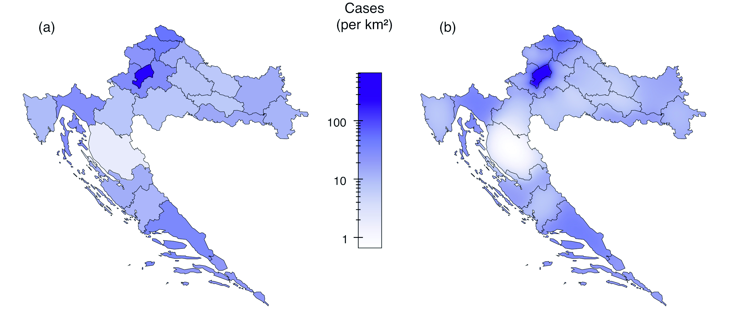
which can be statistically interpreted as imputation of missing data by substituting the mean. Henceforth, we apply equation (4) as a condition on any pycnophylactic density.Figure 1(a) illustrates the definition of ρ plateau, using COVID-19 cases in Croatia between 25 February 2020 and 24 March 2022 (Croatian Institute of Public Health 2022). In this example, the density is obtained by dividing the number of COVID-19 cases in a county by the county’s area. Although ρ plateau is easily calculated, piecewise constant densities are unsuitable statistical models for COVID-19 cases and many other geospatial data because of the discontinuities at the boundaries of enumeration units. As pointed out byOpenshaw (1984): ‘The areal units used to report census data (enumeration districts, census tracts, wards, local government units) have no natural or meaningful geographical identity.’ Thus, to reduce the artefacts introduced by arbitrary boundaries of enumeration units, it is generally preferable to work with a smooth density, as illustrated inFigure 1(b), instead of ρ plateau, whose shape strongly depends on the location of the boundaries.
Figure 1 Two pycnophylactic densities that represent the distribution of COVID-19 cases in Croatia between 25 February 2020 and 24 March 2022. (a) Piecewise constant density. (b) Smooth density obtained from a density-equalising map projection. / Slika 1 Dvije piknofilaktičke funkcije koje prikazuju razdiobu slučajeva bolesti COVID-19 u Hrvatskoj između 25. veljače 2020. i 24 ožujka 2022. (a) po dijelovima konstantna gustoća (b) izglađena gustoća dobivena s pomoću projekcije koja ujednačava gustoću
Tobler (1979a) introduced a cellular automaton algorithm for generating smooth pycnophylactic densities, which approximates the continuum of space with a fine-grained square grid. Each point (x, y) on the grid is initially assigned the density ρ plateau(x, y). Thereafter, the density associated with each grid point is adjusted so that the absolute value of the discrete Laplacian is reduced, subject to the constraints that the sum of densities in each enumeration unit is conserved and density remains nonnegative. This adjustment is iterated until the changes are below a small threshold value or until the number of iterations reaches a predefined limit.
Tobler’s (1979a) algorithm has become the standard technique for smooth pycnophylactic interpolation. The algorithm has been implemented in R (Brunsdon, 2014) and Python (Pysal Developers, 2021). For users of Geographic Information Systems software, the algorithm is also available via extensions of ArcGIS (Qiu et al., 2012) and GRASS (Metz, 2013). A variant ofTobler’s (1979a) algorithm was developed byRase (2001), in which the regular square grid is replaced by an irregular triangular network. However, the algorithm byRase (2001) and its later refinement by the same author(Rase, 2007)keep the essential features ofTobler’s (1979a) algorithm: iterative local averaging and subsequent redistribution of density differences to enforce the pycnophylactic condition of equation (1). Despite the widespread use ofTobler’s (1979a) algorithm, it was not the first method proposed by him for smooth pycnophylactic interpolation. In an earlier publication,Tobler (1976) described an alternative approach in which the boundaries of enumeration units are transformed into an area cartogram (i.e. a map in which all enumeration units are depicted with an area proportional to their population).Tobler’s (1976) proposed method requires the area cartogram to be contiguous; that is, neighbouring enumeration units on the surface of the earth must be neighbours in the cartogram. As noted byTobler (2017), contiguous cartograms are closely related to density-equalising map projections. In this study, we briefly review the connections between contiguous cartograms, density-equalising map projections and smooth pycnophylactic interpolation. Thereafter, we explain how to achieve smooth pycnophylactic interpolation using a recently developed algorithm that generates contiguous cartograms.
2. Relationship Between Pycnophylactic Interpolation and Density-Equalising Map Projections
To construct a contiguous cartogram, the boundaries of enumeration units are modelled as polylines. We denote the vertices of the polylines on an equal-area map projection by (ν1x, ν1y), (ν2x,ν2y), … The vertices are then shifted to new positions (w1x, w1y), (w2x,w2y), … such that the regions demarcated by the transformed boundaries have an area proportional to the population of the corresponding enumeration units. This transformation can be regarded as the result of a map projection t = (tx,ty) that satisfies the conditions tx(vjx,vjx = w jx and ty(vjx,vjx = w jy for all j = 1,2,… A map projection with this property can be obtained, for example, by solving the following equation:
where det Jt = (∂tx/∂x) (∂ty/∂y) - (∂ty/∂x) (∂tx/∂y) is the Jacobian determinant of t, ρ(x, y) is a pycnophylactic density [i.e. it satisfies equation (1)] and ρ_ is its spatial average given by equation (3). The quantity
can then be interpreted as ‘residual density’ (i.e. the difference from the mean density that remains unexplained by the projection t), and the objective is to find a solution t such that ρres(x, y) = 0 for all (x, y).
Contiguous cartograms and density-equalising map projections are related to each other in two ways. First, if ρ and (νjx, νjy) are known, it is possible to solve equation (5) to obtain t(x, y) and then obtain the polyline vertices (wjx, wjy) of a contiguous cartogram by applying t(x, y) to (νjx, νjy) for all j = 1,2,… Second, if (νjx, νjy) and (wjx, wjy) are known, it is possible to construct a density-equalising map projection t(x, y) with the property t(νjx, νjy) = (wjx, wjy) and then obtain a pycnophylactic density by inverting equation (5):
In both cases, solutions are not unique. If ρ(x, y) is given, equation (5) allows infinitely many solutions t(x, y) because the number of constraints implicit in equation (5) is 1, which is less than the number of dimensions (i.e. 2) of a geographic map. Conversely, if all (wjx, wjy) are given, there are infinitely many ways to extend a function t with the property t(vjx, vjy) = (wjx, wjy) to the entire mapping domain. One could impose additional constraints on t(x, y) to make the solution unique. At first glance, an obvious constraint would be to demand that t(x, y) be conformal. However, conformality adds two constraints to the problem in the form of the Cauchy–Riemann equations; hence, together with the constraint of satisfying equation (5), the problem of finding t(x, y) would be overdetermined (Gastner and Newman, 2004). Instead of demanding strict conformality,Tobler (1973) proposed that deviations from conformality should, at least, be minimised when constructing cartograms. However, he reported that a computer program, designed to find nearly conformal density-equalising map projections, failed to converge. Furthermore, it is not evident that a conformal map projection t(x, y) necessarily generates desirable properties for a pycnophylactic density ρ(x, y), calculated using equation (7). Therefore, we describe a method that is guaranteed to find a density-equalising map projection t(x, y) and a smooth pycnophylactic density ρ(x, y), even if neither t(x, y) nor ρ(x, y) satisfy predefined criteria of optimality.
3. Obtaining a Pycnophylactic Interpolation from a Density-Equalising Map Projection
Gastner et al. (2018) introduced a flow-based algorithm that generates density-equalising map projections. In this algorithm, ρ(x, y) in equation (5) is treated as the initial density of a fluid. The algorithm proceeds by constructing a velocity field that conserves the mass of the fluid, is free of vortices and equilibrates the density over time. By integrating the velocity, the algorithm determines the final displacement t(x, y) of any arbitrary point that is initially at position (x, y). It can be shown that t(x, y) satisfies equation (5); thus, t(x, y) is a density-equalising map projection.
For the boundary conditions chosen byGastner et al. (2018), t(x, y) can be calculated efficiently by applying a Fourier transform to the residual density ρ res(x, y). Suppose that ρ(x, y) is initially chosen to be the piecewise constant function ρplateau given by equation (2) on the unprojected map, where det J t = 1 ∀ (x, y). Hence, the initial residual density can be expressed as follows:
where ρ _ is the spatial average, defined in equation (3).Figure 2(a) shows ρres,1(x, y), using COVID-19 cases in Croatia as an example. Because ρres,1(x, y) has discontinuities at the boundaries of enumeration units, the Fourier transform of ρres,1(x, y) exhibits the Gibbs phenomenon (Carslaw 1925); that is, the approximation of ρres,1(x, y) by a finite Fourier series exhibits large oscillations at the boundaries. These oscillations can cause numerical artefacts in subsequent calculations. To circumvent this problem,Gastner’s (2022) computer implementation of the flow-based algorithm removes discontinuities from ρres,1(x, y) by applying Gaussian smoothing as a low-pass filter.Figure 2(b) illustrates the effect of Gaussian smoothing. The density after Gaussian smoothing can be calculated rapidly in Fourier space. However, Gaussian smoothing tends to shift density towards sparsely populated regions; thus, it does not produce a pycnophylactic density. Consequently, the calculated map projection t 1(x, y) is not density-equalising. Nevertheless, by projecting the boundaries, densely populated enumeration units tend to expand, and sparsely populated enumeration units tend to shrink, as shown by the county borders inFigure 2(c). We note that the algorithm replenishes the density that leaks out of the interior of Croatia inFigure 2(b)before calculating the residual density inFigure 2(c).
Figure 2 Steps in the calculation of a pycnophylactic density of COVID-19 cases in Croatia. Starting from an equal-area map in (a), a contiguous cartogram is iteratively calculated in (b) to (f). Panels (b),(d) and (f) show the residual density after Gaussian smoothing of the densities shown in (a), (c) and (e), respectively. / Slika 2 Koraci pri računanju piknofilaktičke funkcije za slučajeve bolesti COVID-19 u Hrvatskoj. Počevši s kartom u ekvidistantnoj projekciji (a), kartogrami susjedstva se iterativno računaju (b) − (f). Slike (b),(d) i (f) pokazuju rezidualnu gustoću nakon Gaussova izglađivanja gustoća prikazanih na slikama (a), (c) i (e).
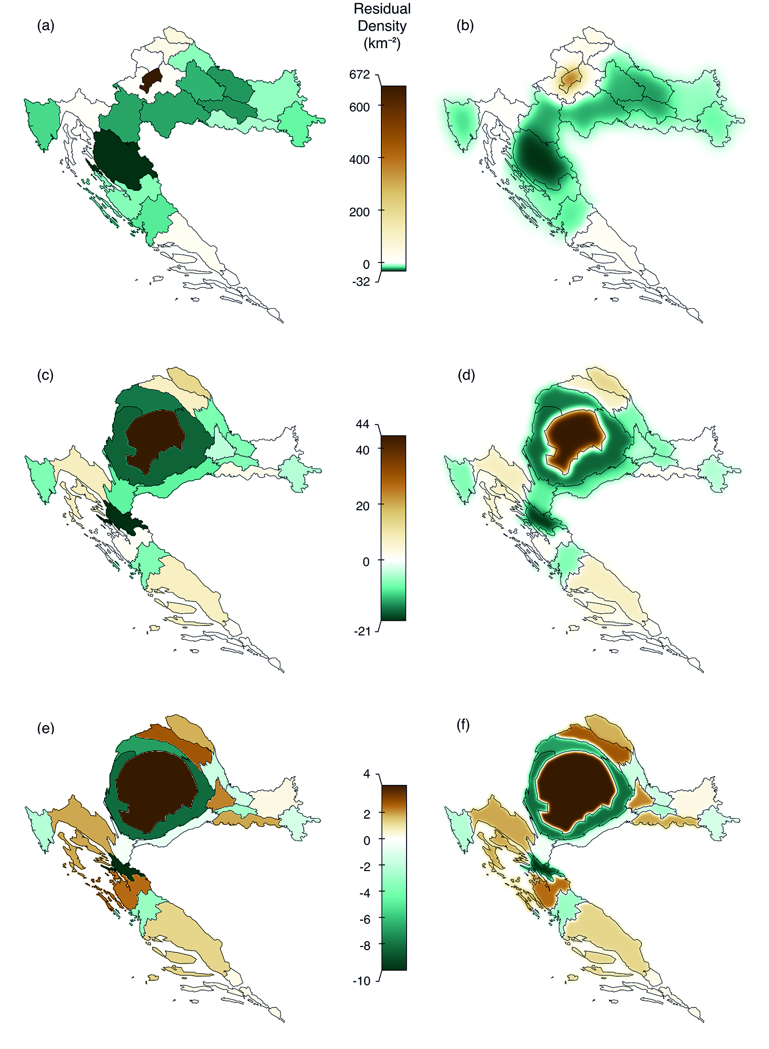
To improve density-equalisation, the computer program byGastner (2022) inserts the boundaries obtained from the initial run of the flow-based algorithm as input into a second run; that is, a new piecewise constant residual density ρ res,2(x, y) is constructed; Gaussian smoothing is applied to ρ res,2(x, y), as indicated inFigure 2(d); and a new projection t 2(x, y) is calculated. The newly projected boundaries, shown inFigure 2(e), can be reinserted into the algorithm, which again calculates a piecewise constant residual density ρres,3(x, y) before applying Gaussian smoothing, as shown inFigure 2(f). With each iteration k, discontinuities of ρres,k(x, y) tend to become smaller. Thus, the width of the Gaussian kernel that is used for smoothing can be made smaller after each iteration until the width becomes indistinguishable from zero. The colour bars inFigure 2 show that the residual density converges towards zero as the procedure is repeated.
Denoting the projections calculated in the k-th iteration of the flow-based algorithm by t k(x, y), a solution to equation (2) can be obtained by the function composition t(x, y) = t l ∘ t l-1 ∘ … ∘ t1(x, y), provided that l is sufficiently large. In practice, values of l between 5 and 20 are usually sufficient to make the areas of all enumeration units on the cartogram accurate to within 1%. The composed projection t(x, y) is differentiable at the boundaries of the enumeration units because each projection \mathbf{t}_k(x,y) is the result of Gaussian convolution and, hence, differentiable (Gwosdek et al. 2012). The computer program approximates the Jacobian determinant det Jt as the factor by which the areas of cells in a fine-grained square grid increase (det Jt > 1) or decrease (det Jt < 1) because of t(x, y). In the case of Croatia, the program uses a grid with 512 horizontal and 512 vertical lines. Afterwards, equation (7) is used to solve for ρ(x, y), which results in a finite-size approximation of a differentiable pycnophylactic density.Figure 1(b) shows the result for COVID-19 cases in Croatia.
4. Conclusion
The program byGastner (2022) is written in C++ and optimised for computational speed. For the map shown inFigure 1(b), the calculation needed only an average time of 5.1 seconds for a test run on a MacBook Pro laptop with a 2.7 GHz Quad-Core Intel i7 processor. We acknowledge that a comparison withTobler’s (1979a) algorithm would require careful benchmarking of run times, which we still need to implement. However, our preliminary studies suggest that the method described above requires fewer iterations thanTobler’s (1979a) algorithm. This observation is explained by the fact that, in the cartogram-based algorithm outlined above, the density associated with any point in space already changes after the first iteration, even for points far from any boundary, because of the significant width of the initial Gaussian kernel. By contrast, inTobler’s (1979a) algorithm, a grid point that is m grid spacings away from the nearest boundary requires O(m) iterations until its density is affected by a neighbouring enumeration unit. This advantage of the cartogram-based algorithm is partly offset by the time needed to calculate Fourier transforms. However, we hypothesise that the substantial reduction in the number of overall iterations more than compensates for the cost of the Fourier transforms. AsTobler (1979b) himself noted, ‘The use of a fast Fourier transform … should be investigated to hasten convergence of the algorithm.’
We also acknowledge that pycnophylactic densities generated by the algorithm outlined above do not optimise any predefined criterion for smoothness, whereasTobler’s (1979a) algorithm directly minimises ∬[( ∂ 2 ρ/∂x2 + ∂ 2 ρ/∂y2)2]dxdy. However, the density ρ obtained from our algorithm could be used as input toTobler’s (1979a) algorithm, thereby combining the benefits of both methods. The potential advantages of combining the algorithms will be investigated in future work.
1. Uvod
Kvantitativni geoprostorni podatci često su dostupni samo kao agregirani brojevi za diskretne popisne jedinice. Na primjer, nacionalne statističke agencije obično izvještavaju o broju pojedinaca koji žive u svakoj administrativnoj podjeli zemlje (npr. popisni blok u Sjedinjenim Državama i izlazno područje u Ujedinjenom Kraljevstvu), ali ne objavljuju informacije o točnoj lokaciji svakog pojedinca. Budući da je nemoguće imati točne lokacije, agregirani podatci često se pretvaraju u funkciju gustoće (u jedinicama ljudi po kvadratnom kilometru) koja svakoj točki koja pripada kontinuumu koordinata dodjeljuje realni broj. Pretpostavimo da je država podijeljena na popisne jedinice U1, ..., Un. Označimo broj stanovnika u Ui s Pi, a površinu s Ai. Nadalje, pretpostavljamo da su koordinate već konvertirane iz geografskih u kartezijeve (x, y) upotrebom neke ekvivalentne projekcije. Omeđena, nenegativna funkcija ρ(x, y) je piknofilaktička ili piknofilaksa (od grčke riječi πυκνός, što znači ‘gust’, i φύλαξ, što znači ‘čuvar’) ako je agregirana gustoća u Ui jednaka opažanoj populaciji Pi:
Varijabla P_i ne mora biti populacija u uskom smislu; može se odnositi na druge podatke koji su dostupni u agregiranom obliku (npr. bruto regionalni proizvod ili emisije CO2 po popisnim jedinicama). Zbog toga se u nastavku koristimo nazivom ‘populacija’ za bilo koji tip nenegativnih, prostorno agregiranih podataka.
Primjer piknofilaktičke funkcije je ova po dijelovima konstantna funkcija:
gdje je
prostorno osrednjena gustoća. U principu, gustoća izvan svih popisnih jedinica može se odabrati proizvoljno jer se ne može zaključiti iz dostupnih podataka. Međutim, pokazalo se da je matematički zgodno zadati uvjet
što se može statistički protumačiti kao imputacija podataka koji nedostaju zamjenom srednje vrijednosti. Od sada nadalje primjenjujemo jednadžbu (4) kao uvjet na bilo koju piknofilaktičku funkciju.Slika 1(a) ilustrira definicijuρplateau, koristeći slučajeve bolesti COVID-19 u Hrvatskoj u razdoblju od 25. veljače 2020. do 24. ožujka 2022. (Hrvatski zavod za javno zdravstvo 2022). U tom primjeru, gustoća se dobiva dijeljenjem broja slučajeva bolesti COVID-19 u županiji s površinom županije. Iako se ρplateau lako izračunava, po dijelovima konstantne gustoće neprikladni su statistički modeli za slučajeve bolesti COVID-19 i mnoge druge geoprostorne podatke zbog diskontinuiteta na granicama popisnih jedinica. Kao što je istaknuoOpenshaw (1984): "Površinske jedinice koje se koriste za izvješćivanje popisnih podataka (popisna područja, okruzi, jedinice lokalne samouprave) nemaju prirodni ili smisleni geografski identitet." Dakle, da bi se smanjili artefakti koji se unose zbog proizvoljnih granica popisnih jedinica, općenito je poželjno raditi s glatkom gustoćom, kao što je prikazano naslici 1(b), umjestoρplateau, čiji oblik jako ovisi o položaju granica.
Tobler (1979a) je uveo algoritam staničnog automata za generiranje glatkih piknofilaktičkih funkcija koje aproksimiraju kontinuum prostora s finom kvadratnom mrežom. Svakoj točki (x, y) te mreže pridružena je inicijalno gustoća ρplateau(x, y). Nakon toga, gustoća povezana sa svakom točkom mreže prilagođava se tako da se apsolutna vrijednost diskretnog Laplaceana smanjuje, podložno ograničenjima da se zbroj gustoća u svakoj popisnoj jedinici čuva i da gustoća ostaje nenegativna. Ta se prilagodba ponavlja sve dok promjene nisu ispod male vrijednosti praga ili dok broj iteracija ne dosegne unaprijed definirano ograničenje.
Toblerov (1979a) algoritam postao je standardna tehnika za glatku piknofilaktičku interpolaciju. Algoritam je primijenjen u R-u (Brunsdon 2014) i Pythonu (Pysal Developers 2021). Za korisnike softvera za GIS algoritam je također dostupan preko proširenja ArcGIS-a (Qiu i dr. 2012) i GRASS-a (Metz 2013). VarijantuToblerova (1979a) algoritma razvio jeRase (2001), pri čemu je pravilna kvadratna mreža zamijenjena neregularnom mrežom trokuta. Međutim,Raseov algoritam (2001) i kasnija profinjenja istog autora (Rase 2007) zadržala su bitna svojstvaToblerova (1979a) algoritma: iterativno lokalno usrednjavanje i naknadna preraspodjela razlika u gustoći kako bi se učvrstio piknofilaktički uvjet (1). Unatoč raširenoj upotrebiToblerovog (1979a) algoritma, to nije bila prva metoda koju je on predložio za glatku piknofilaktičku interpolaciju. U ranijoj publikaciji,Tobler (1976) je opisao alternativni pristup u kojem se granice popisnih jedinica pretvaraju u površinski kartogram (tj. kartu u kojoj su sve popisne jedinice prikazane s površinom proporcionalnom njihovoj populaciji). PredloženaToblerova metoda (1976) zahtijeva da površinski kartogram područja bude susjedan; odnosno susjedne popisne jedinice na Zemljinoj površini moraju biti susjedi na kartogramu. Kao što je primijetioTobler (2017), kartogrami susjedstva usko su povezani s kartografskim projekcijama s ujednačavanjem gustoće. U ovom članku ukratko opisujemo veze između kartograma susjedstva, kartografskih projekcija s ujednačavanjem gustoće i glatke piknofilaktičke interpolacije. Nakon toga objašnjavamo kako postići glatku piknofilaktičku interpolaciju koristeći nedavno razvijeni algoritam koji generira kartograme susjedstva.
2. Odnos između piknofilaktičke interpolacije i kartografske projekcije s ujednačavanjem gustoće
Da bi se konstruirao kartogram susjedstva granice popisnih jedinica se modeliraju kao polilinije. Označimo vrhove polilinija u nekoj ekvivalentnoj projekciji s (v1x,v1y), (v2x,v2y),... Vrhovi se onda pomaknu u nove položaje (w1x,w1y), (w2x,w2y), ... tako da regije razgraničene transformiranim granicama imaju površinu proporcionalnu populaciji odgovarajućih popisnih jedinica. Ta transformacija može se doživjeti kao kartografska projekcija t = (tx, ty) koja zadovoljava uvjete tx(vjx,vjy) = wjx i ty(vjx,vjy) = wjy za svaki j = 1,2,... Kartografska projekcija s takvim svojstvom može se dobiti, na primjer, rješavanjem jednadžbe:
gdje je det Jt = (∂tx/∂x)(∂ty/∂y) - (∂ty/∂x)(∂tx/∂y) Jacobijeva determinanta od t, ρ(x, y) je piknofilaktička funkcija [zadovoljava jednadžbu (1)] i ρ_ je njezina prostorna sredina dana jednadžbom (3). Veličina
može se interpretirati kao "rezidual gustoće" (tj. razlika između srednje gustoće koja ostaje neobjašnjena projekcijom t), a cilj je naći rješenje t tako da bude ρres = 0 za sve (x, y).
Kartogrami susjedstva i kartografske projekcije koje ujednačuju gustoću međusobno se odnose na dva načina. Prvo, ako su ρ i (vjx,vjy) poznati, moguće je riješiti jednadžbu (5) da se dobije t(x, y) i onda dobiti vrhove polilinije (wjx,wjy) kartograma susjedstva primijenjujući t(x, y) na (vjx,vjy) za sve j = 1,2,... Drugo, ako (vjx,vjy) i (wjx,wjy) nisu poznati, moguće je konstruirati kartografsku projekciju s ujednačenom gustoćom t(x, y) sa svojstvom t (vjx,vjy) = (wjx,wjy) i onda dobiti piknofilaktičku funkciju invertiranjem jednadžbe (5):
U oba slučaja rješenje nije jedinstveno. Ako je zadano ρ(x, y), jednadžba (5) daje beskonačno mnogo rješenja t(x, y) jer je broj uvjeta sadržanih u jednadžbi (5) jednak 1, što je manje od dimenzija karte (tj. 2). Obratno, ako su zadani svi (wjx,wjy), tada postoji beskonačno mnogo načina za proširenje funkcije t sa svojstvom t (vjx,vjy) = (wjx,wjy) na cijelom području definicije preslikavanja. Da bi se dobilo jedinstveno rješenje mogu se na t(x, y) postaviti dodatni uvjeti. Na prvi pogled, jedan očiti uvjet mogao bi biti zahtjev da je preslikavanje t(x, y) konformno. Međutim, konformnost dodaje dva uvjeta u obliku Cauchy–Riemannovih jednadžbi; zbog toga, zajedno s uvjetom zadovoljavanja jednadžbe (5), problem pronalaženja t(x, y) bio bi preodređen (Gastner i Newman 2004). Umjesto traženja striktne konformnosti,Tobler (1973) je predložio da odstupanja od konformnosti trebaju barem biti minimizirana pri konstrukciji kartograma. Međutim, on je izvijestio da računalni program oblikovan za pronalaženje skoro konformnih projekcija s ujednačenjem gustoće ne konvergira. Nadalje, nije očito da konformna projekcija t(x, y) nužno generira poželjna svojstva piknofilaktičke funkcije ρ(x, y), izračunane s pomoću jednadžbe (7). Dakle, mi opisujemo metodu koja garantira pronalaženje projekcije t(x, y) koja ujednačuje gustoće i glatku piknofilaktičku funkciju ρ(x, y), čak i ako ni t(x, y) ni ρ(x, y) ne zadovoljavaju unaprijed definiran kriterij optimalnosti.
3. Dobivanje piknofilaktičke interpolacije iz projekcije koja ujednačuje gustoću
Gastner i dr. (2018) uveli su algoritam utemeljen na toku koji generira projekcije koje ujednačuju gustoću. U tom algoritmu, ρ(x, y) u jednadžbi (5) tretira se kao početna gustoća fluida. Algoritam nastavlja s konstrukcijom polja brzina koje čuva masu fluida, bez vrtloga je i uravnotežuje gustoću tijekom vremena. Integriranjem brzine algoritam određuje konačni pomak t(x, y) proizvoljne točke koja je u početnom položaju (x, y). Može se pokazati da t(x, y) zadovoljava jednadžbu (5); dakle t(x, y) je projekcija koja ujednačuje gustoću.
Za rubne uvjete koje su izabraliGastner i dr. (2018), t(x, y) se može učinkovito izračunati primjenom Fourierove transformacije na rezidualnu gustoću ρres. Pretpostavimo da je ρ(x, y) početno odabrana kao po dijelovima konstantna funkcija ρplateau zadana jednadžbom (2) na neprojiciranoj karti, gdje je det Jt1,∀(x, y). Zato se početna rezidualna gustoća može izraziti ovako:
gdje je ρ_ prostorna sredina definirana jednadžbom (3).Slika 2(a) pokazuje primjer ρres,1(x, y) za slučajeve bolesti COVID-19 u Hrvatskoj. Budući da ρres,1(x, y) ima diskontinuitete na granicama popisnih jedinica, Fourierova transformacija od ρres,1(x, y) pokazuje Gibbsov fenomen (Carslaw 1925); tj. aproksimacija od ρres,1(x, y) primjenom konačnih Fourierovih redova daje velike oscilacije na granicama. Te oscilacije mogu prouzročiti numeričke artefakte pri računanjima koja slijede. Da bi se to izbjeglo,Gastnerova (2022) računalna primjena algoritma utemeljnog na toku uklanja diskontinuitete od ρres,1(x, y) primijenjujući Gaussovo izglađivanje kao niskopropusni filter.Slika 2(b) ilustrira učinak Gaussovog izglađivanja. Nakon Gaussova izglađivanja gustoća se može brzo izračunati u Fourierovu prostoru. Međutim, Gaussovo izglađivanje ima tendenciju pomaka gustoće prema slabije popunjenim područjima; dakle, ono ne daje piknofilaktičku funkciju. Prema tome, izračunana projekcija t1(x, y) ne ujednačuje gustoću. Bez obzira na to, projiciranjem granica, gusto naseljene popisne jedinice imaju tendenciju širenja, a rijetko naseljene popisne jedinice imaju tendenciju smanjivanja, kao što pokazuju granice županija naslici 2(c). Uočimo da algoritam nadopunjuje gustoću koja curi iz unutrašnjosti Hrvatske naslici 2(b) prije nego što izračuna zaostalu gustoću naslici 2(c).
Kako bi poboljšao ujednačavanje gustoće,Gastnerov računalni program (2022) umeće granice dobivene iz početnog pokretanja algoritma temeljenog na protoku kao ulaz u drugu iteraciju; tj. konstruirana je nova po dijelovima konstantna rezidualna gustoća ρres,2; Gaussovo izglađivanje je primijenjeno na ρres,2, kao što je prikazano naslici 2(d); i izračuna se nova projekcija t2(x, y). Nove granice, prikazane naslici 2(e), mogu se ponovno staviti u algoritam, koji ponovno računa po dijelovima konstantnu rezidualnu gustoću ρres,3(x, y) prije primjene Gaussova izglađivanja, kako je prikazano naslici 2(f). Sa svakom iteracijom k, diskontinuiteti od ρres,k(x, y) postaju sve manji. Dakle, širina Gaussove jezgre koja se koristi za izglađivanje može se nakon svake iteracije smanjiti sve dok širina ne postane nerazlučiva od nule. Trake u boji naslici 2 pokazuju da se zaostala gustoća približava nuli kako se postupak ponavlja.
Označimo li projekciju izračunanu u k-toj iteraciji algoritma utemeljenog na toku s tk(x, y), rješenje jednadžbe (2) može se dobiti kao kompozicija funkcija t(x, y) = tl ∘ tl-1 ∘ ... ∘ t1(x, y), uz pretpostavku da je l dovoljno velik. U praksi su vrijednosti l između 5 i 20 obično dovoljne da površine svih popisnih jedinica na kartogramu budu točne na 1%. Složena funkcija t(x, y) je diferencijabilna na granicama popisnih jedinica jer je svaka projekcija \mathbf{t}_k(x,y) rezultat Gaussove konvolucije i stoga diferencijabilan (Gwosdek i dr. 2012). Računalni program aproksimira Jacobijevu determinantu det Jt kao faktor s pomoću kojeg površine fine kvadratne mreža povećavaju (det Jt > 1) ili smanjuju (det Jt < 1) zbog t(x, y). U slučaju Hrvatske program upotrebljava mrežu od 512 horizontalnih i 512 vertikalnih linija. Nakon toga, p(x, y) se dobije rješavanjeme jednadžbe (7) što rezultira aproksimacijom diferencijabilne piknofilaktičke funkcije.Slika 1(b) pokazuje rezultat slučajeva bolesti COVID-19 za Hrvatsku.
4. Zaključak
Gastnerov program (2022) napisan je u C++ i optimiran za brzinu računanja. Za kartu prikazanu naslici 1(b), računanje je trajalo oko 5,1 sekundi za testiranje na laptopu MacBook Pro s procesorom 2.7 GHz Quad-Core Intel i7. Potvrđujemo da bi usporedba sToblerovim (1979a) algoritmom zahtijevala pažljivu usporedbu vremena izvođenja, što planiramo napraviti. Međutim, naše preliminarne studije sugeriraju da naša metoda zahtijeva manje ponavljanja negoToblerov (1979a) algoritam. To opažanje objašnjava se činjenicom da se u algoritmu koji se temelji na kartogramu gustoća povezana s bilo kojom točkom u prostoru već mijenja nakon prve iteracije, čak i za točke udaljene od bilo koje granice, zbog značajne širine početne Gaussove jezgre. Nasuprot tome, uToblerovom (1979a) algoritmu točka mreže koja je udaljena m razmaka mreže od najbliže granice zahtijeva O( m) iteracija sve dok na njezinu gustoću ne utječe susjedna popisna jedinica.
Ova prednost algoritma zasnovanog na kartogramu djelomično je nadoknađena vremenom potrebnim za izračunavanje Fourierovih transformacija. Međutim, pretpostavljamo da značajno smanjenje broja ukupnih iteracija više nego kompenzira trošak Fourierovih transformacija. Kao što je samTobler (1979b) primijetio: "Upotrebu brze Fourierove transformacije... treba istražiti kako bi se ubrzala konvergencija algoritma."
Također potvrđujemo da piknofilaktike generirane našim algoritmom ne optimiraju nijedan unaprijed definirani kriterij za glatkoću, dokToblerov (1979a) algoritam izravno minimizira ∬[(∂2p/∂x2 + ∂2p/∂y2)2]dx dy. Međutim, gustoća p dobivena iz našeg algoritma mogla bi se koristiti kao ulaz uToblerov (1979a) algoritam, kombinirajući na taj način prednosti obje metode. Potencijalne prednosti kombiniranja algoritama istraživat će se u budućem radu.
