1. Introduction
Three-dimensional reconstruction refers to the reconstruction of three-dimensional space coordinates and gestures of objects from images or videos[1]. In the process of 3D reconstruction model construction, the common methods include the sensor method and deep learning method. Among them, sensor methods usually require the use of hardware devices such as optical sensors or cameras to obtain image or video data. However, these devices are often expensive and cannot be processed in real time[2]. Therefore, most research uses deep learning models for 3D reconstruction. Recently, the use of network structures such as neural networks and attention mechanisms attention techniques is common. Many studies have shown that the use of neural networks and attention mechanisms can optimize ordinary models to capture better global image features and information[3]. Based on this background, a 3D reconstruction model based on the Convolutional Block Attention Module (CBAM) model and multi-view stereo vision framework is proposed in this study. The model first uses the CBAM to capture the relationship between the important information and local features in the image and then it uses the multi-view stereo vision framework to construct the 3D reconstruction model. The innovations of this research are mainly reflected in the following aspects. First, the spatial attention mechanism and channel attention mechanism are innovatively combined and applied to the field of 3D reconstruction, which significantly improves the model's ability to capture local features by fine-tuning the model's attention to the important information in the image, thus realizing higher reconstruction accuracy without sacrificing the reconstruction speed. Secondly, based on the multi-view stereo vision algorithm, the fusion processing of the algorithm on image features from different viewpoints is optimized through the introduction of CBAM, which enhances the model's adaptability and reconstruction effect on complex scenes. Finally, through extensive testing on several recognized datasets, this study not only compares the performance differences between the model and existing techniques but also analyzes in depth the specific contribution of the CBAM to the model's performance enhancement and provides detailed experimental results and analyses to prove the effectiveness and superiority of the proposed method. Through these innovations, this study achieves significant improvements in the accuracy, efficiency, and application range of 3D digital image virtual scene reconstruction, providing new ideas and technical support for subsequent related research. This research is divided into four parts: First, the summary of other people's research; Second, the paper discusses the main methods. Then, the model performances are tested Finally, the experimental conclusions and future research directions are presented.
2. Related work
Attentional mechanisms are a key intelligence technique mainly used to enhance the ability of deep learning models to process data by focusing on important information in order to improve the performance of tasks such as natural language processing and image recognition. Multi-view stereo vision, on the other hand, encompasses a range of AI techniques that reconstruct the 3D form of an object by analyzing images taken from multiple angles and is widely used in areas such as 3D reconstruction, robot navigation, and augmented reality. Both techniques play an important role in the field of artificial intelligence, especially in improving the accuracy and efficiency of image processing and computer vision applications[4]. Yao et al. combined a deep learning network and attention mechanism to build a system to simulate visual scenes and realized the prediction function of the change attributes of simulated visual scenes. This system can be of high application value in simulating visual scenes and can effectively predict the changing attributes of scenes[5]. To effectively detect the blade cracks of aero engines, Hui et al. constructed a Yolov4-tiny model using an improved attention mechanism and added a bi-cubic interpolation function to the model. This model can not only reduce the interference of redundant detection results but also increase the detection accuracy by 12.3% compared with the traditional Yolov4-tiny model[6]. Tian et al. applied an attention mechanism to skin image diagnosis. The model first uses a multi-view convolutional neural network to extract information from skin pigmentation images, and then uses an attention mechanism to analyze the extracted data and deeply studies the main factors affecting the diagnosis of pigmentation. This method is advanced and can effectively diagnose pigmentation in skin images[7]. Yao et al. applied the attention mechanism to the defect diagnosis of knitted clothing. Firstly, the proposed frames of knitted clothing defect types were constructed by the attention mechanism network, and then the region-specific diagnosis aggregation method was used to map the clothing defects into the feature map. Finally, the defects were classified according to their features. The detection speed of this framework is 0.085s, and the average detection accuracy is 0.9338[8]. Zhang et al. suggested a multipath attention mechanism algorithm. The proposed algorithm can strengthen the association between image features and increase the function of recognizing the structural data between different scales. Experimental results verify the excellence of this algorithm[9]. To improve the optimization effect in stereoscopic images, Lyons et al. adopted multi-view stereoscopic algorithms with different Field of View (FOV) widths for research. Although a larger FOV width can improve the angle recognition performance of the multi-view stereo algorithm for stereoscopic images, the overall performance will be relatively reduced, so the setting of FOV width will affect the application performance of the multi-view stereo algorithm[10]. Li et al. used deep learning network and multi-view stereo vision to build a stereo tracking system for the human body and integrated the segmentation results into the 3D model to achieve stereo recognition. This system can not only effectively resist external interference for human body image recognition but also has high computational performance[11]. Guo et al. proposed a single view block detection method for stereo image matching, which not only effectively avoids the recognition error of stereo image occlusion position but also improves the image matching effect. This method has a small error in stereo image recognition[12].
To sum up, both the attention mechanism algorithm and the multi-view stereo vision algorithm have deep applications in different fields. However, the above two algorithms are still rarely applied in the field of 3D digital image virtual scene reconstruction[13]. In this study, the CBAM with good feature extraction and depth operation function and multi-view stereo vision algorithm were combined to build a model.
3.Design of 3D digital image virtual scene reconstruction algorithm based on machine learning technology
To optimize the traditional 3D reconstruction algorithm, this paper first introduces the relevant steps of the 3D reconstruction algorithm and then adopts the multi-view stereo vision to reconstruct the 3D model. Aiming at the defects of multi-view stereo vision algorithm in extracting image features, this paper combines the Spatial Attention Mechanism (SAM) and CAM and finally generates a CBAM. This mechanism is applied to the multi-view stereo vision algorithm model to enhance the image processing effectiveness of the 3D reconstruction method.
3.1 Research on 3D reconstruction algorithm
3D reconstruction refers to the technology of rebuilding and simulating the 3D model of the physical world through algorithms. Ordinary 3D reconstruction algorithms include 3D image matching, 3D point cloud model matching, 3D model reconstruction, etc.[14]. The above algorithms can be used in virtual reality, augmented reality, autonomous driving, game development, and other fields. Traditional 3D reconstruction mainly uses visual technology to build the model. The specific data graphics of the scene body are obtained by the camera. The obtained images are analyzed and processed and then fused with computer vision knowledge to deduce the three-dimensional information of objects in the display environment. The flow chart of traditional 3D reconstruction technology is shown in Figure 1[15].
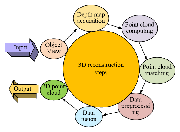
Fig. 1 Flow chart of 3D reconstruction
Figure 1 shows the 3D reconstruction process. The complete 3D reconstruction flow chart includes five steps: depth map acquisition, image pre-processing, point cloud computing, point cloud registration, and data combination. Among them, the depth map needs to be obtained by the depth camera. Just like a normal camera, shooting the environment will still obtain a color image of the environment. If the environment is photographed from different perspectives, then all information about the environment can be obtained. The pre-processing of image data is limited by the resolution of equipment, and there are many shortcomings in the process of acquiring depth map information. The Gaussian filter and median filter are usually used for noise reduction. The essence of the Gaussian filtering method is to carry out a weighted average of pixels. The larger the distance between the target pixel and the comparison pixel, the larger the weight, and Eq. (1) shows its weight equation:
(1)
In Equation (1), w(i, j) denotes the weights of the filter at (i, j). denotes the coefficients of the classical Gaussian weighting function. d’ denotes the distance between the target pixel point and the surrounding pixel points. δ is the standard deviation. e is the base of the natural logarithm.
The median filtering method is the average pixel value obtained after sorting the size pixels of the pixel value, and the image equation after filtering is shown in Eq. (2):
(2)
In Equation (2), g(x, y) represents the filtered image, f(x, y) is the depth image, and W is the two-dimensional median filter template. Point cloud computing can reconstruct a three-dimensional model of the real world. Point cloud computing in the point cloud model refers to the parallel processing of point cloud data, calculating the three-dimensional coordinates of each point, and calculating the cloud model of the point according to these coordinates. Point cloud matching refers to matching a point cloud dataset with a 3D model of the real world to determine the 3D coordinates of each point and its location in the cloud model. Point cloud matching is a key technology in 3D reconstruction models, which can enhance the precision and reliability of 3D reconstruction models. Through point cloud matching, the interaction between the real world and the virtual world can be realized to build a more realistic virtual world. Data fusion is the fusion and filtering of depth maps from different reference views into a dense point cloud, where the conversion equation between image coordinates and world coordinates is shown in Eq. (3):
(3)
In Equation (3), Pω denotes the coordinates of pixels in the image coordinate system. Px denotes the coordinates of pixels in the world coordinate system. T and K are respectively camera internal and external parameter matrices. d denotes the depth value. In the coordinate transformation process of Eq. (3), the depth value is first obtained from the depth map. Next, the pixel coordinates (xi, yi) in the image coordinate system are transformed to the world coordinate system by the depth value and the inner and outer camera parameter matrices, i.e., the pixel coordinates become (Xi, Yi, Zi). The inner parameter matrices contain the camera's focal length and principal point coordinates as the parameters used to transform the 3D coordinates to the 2D image plane coordinates. The outer parameter matrix describes the position and rotation of the camera concerning the world coordinate system and is the matrix used to describe the relationship between the 3D world coordinates and the camera coordinate system. The use of inverse matrices ensures that the conversion of the coordinate system can be accomplished successfully even if the dimensions of the 2D image coordinate system and the 3D world coordinate system do not match.
In the merged point cloud, not all pixels can be saved. To solve this problem, the Multiple View Stereo (MVS) algorithm was used to reconstruct the 3D model. MVS can filter the depth map. For each depth map, a corresponding confidence map is generated. The mapping process is shown in Figure 2.
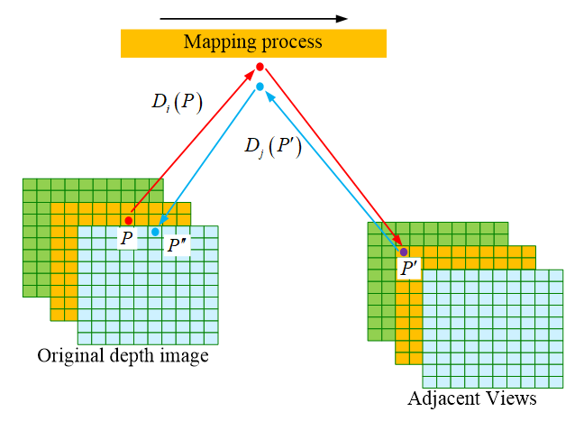
Fig. 2 Depth image pixel map
Figure 2 shows the pixel mapping process of the depth map. Point P in Figure 2 represents pixels of the depth map. Ii represents the original depth image; Ij indicates the mapped adjacent view. By estimating depth Di(P), a pixel P in the image Ii is mapped to another adjacent view Ij, and a new pixel P’ is obtained. The calculation equation of the pixel threshold of the depth map is shown in Eq. (4):
(4)
In Equation (4), τ1 is the threshold value, and P’’ represents another position of point P in the original depth image. Another threshold τ2 is defined as shown in Eq. (5):
(5)
In Equation (5), τ2 represents another threshold, and Dj(P’’) is the projected depth of P’’. Since Ij also has its depth map, the corresponding depth Dj(P’) can also be obtained. According to Eq. (4) and Eq. (5), the filter constraint equation of the depth map can be further obtained. Only pixels that meet the above constraints under at least three adjacent views can be identified as valid pixels.
The indexes to measure the performance of the 3D reconstruction algorithm usually include precision and point cloud integrity. The accuracy calculation equation is shown in Eq. (6):
(6)
Equation (6) is the calculation equation for the accuracy of the 3D reconstruction algorithm. Pp represents the position of any point cloud in the 3D reconstruction model, and Pg is the true value point cloud convergence. Argmin specifies the value of the relevant argument to minimize the following equation. In Eqs. (6) and (7), λ represents the regularization parameter, which is used to balance the weights between the different terms in the model to ensure that the model accurately captures the features of the data without overfitting. Although the F-score is also a commonly used metric to measure the balance between precision and recall in classification problems, in the 3D reconstruction scenario of this study, the average error provides a more intuitive representation of the model's ability to capture the spatial geometry, and thus the final choice is to use the average value to evaluate the model performance.
Integrity refers to the percentage measure of pixel points that can be matched in the reconstructed point cloud of the truth-valued three-dimensional point cloud, and its calculation equation is shown in Eq. (7):
(7)
In Equation (7), is the set of truth-valued point clouds, and the integrity can also be measured by the absolute average distance.
3.2 Construction of 3D digital image virtual scene reconstruction model based on improved MVSNet
MVS is an ordinary computer vision algorithm. This algorithm can obtain images from multiple perspectives and calculate pixels of each image to form a 3D reconstruction model, which is mainly used in the fields of robot vision, 3D reconstruction, games, and visual monitoring[16]. The basic principle of the MVS algorithm is to splice images from multiple perspectives together, determine the pixels of the image by calculating the matching points between each image, and then use these pixels to reconstruct the entire image area. Compared with a single-view algorithm, the MVS algorithm has higher accuracy and reliability and can deal with complex illumination changes and background interference. In addition, the MVS algorithm can reduce computing cost and time and improve computing efficiency. To further enhance the effectiveness of the MVS algorithm, scholars built the Multiple View Stereo Network (MVSNet) model using a deep learning model. Figure 3 shows the MVSNet model.
In Figure 3, the traditional MVSNet model mainly consists of four parts: input view, shared weight, homologous transformation, and aggregate cost. In the MVSNet model, different views are treated as reference views. The neighboring graph of each reference view is also called the source view, and the number of inputs for the source view depends on the case. When the source view and reference view are input into the network simultaneously, they can generate corresponding feature maps according to the feature extraction network of shared weights and then form the feature maps in the reference view space through homologous transformation. The feature graph in the reference space is matched with the feature graph in the source view by similarity to form the aggregate cost. The final refined depth map can be obtained through further processing of the polymerized cost.
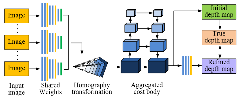
Fig. 3 MVSNet model structure diagram
While MVSNet improves the overall integrity of the scene, it sacrifices the integrity of the local textures. The reason for this is that the function of the feature extraction network is ignored. Therefore, this research combines the SAM and the CAM and finally generates the CBAM, which is used in MVSNet, aiming to improve the feature extraction ability of MVSNet feature extraction network, so as to build the virtual scene reconstruction model of 3D digital image with better effect.
Through the association function, all the source views become views on the principal axis of the reference perspective, which can be represented by a 3×3 matrix, which is obtained by Eq. (8)[17]:
(8)
In Equation (8), Ri denotes the rotation matrix of the source view; Ki is the parameter matrix of the camera; ti denotes the translation matrix of the source view; Hi(d) is the depth of the corresponding spindle space mapped from the source view to the reference view. The overall transformation process is similar to the traditional plane scanning method, after which the specific depth position of each source view on the principal axis of the reference view is obtained. After transformation, the feature vertebra in the reference view is shown in Figure 4.
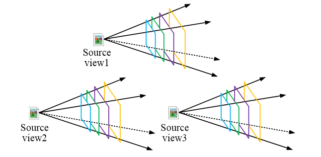
Fig. 4 Improved MVSNet modeling of feature vertebrae on the transformed reference view
The feature vertebrae on the reference view after the transformation of the improved MVSNet model are shown in Figure 4. Like the single reactivity matrix in the traditional method, the transformation matrix applied by MVSNet is also a 3×3 matrix representing the transformation from the image coordinate system to the world coordinate system. The overall transformation process is similar to the traditional planar scanning method, and the specific depth position of each source view on the reference view principal axis is obtained after the transformation. The feature vertebrae of three different source view feature maps are given in Figure 4. As can be seen from Figure 4, the different source view feature maps correspond to the conical space where the reference view is located, but due to the various depth positions where they are located, the views are transformed into the structure of a vertebra for the shooting spindle within the reference view. Since the input of the vertebrae is difficult to fit into the 3D structure, the transformed source view feature maps will be interpolated bilinearly to obtain feature maps with the same length and width. Since the feature map filters the image information and enhances the image features while removing some useless information, the linear interpolation using the feature map is much better than the original 2D image. This step realizes the conversion from 2D to 3D and at the same time encodes the uni-responsive transformation into the network, making the end-to-end training process possible.
Before the homologous transformation, the feature extraction of each input reference view and source view is carried out, and the MVSNet model is used as the basic network structure. Then, the channel attention module is added to the last four layers of feature extraction, and the view image that has not been transformed by homography is sent into the global maximization pool based on image width and height, as shown in Eq. (9):
(9)
In Equation (9), FMax is the maximization pool; Fi is a view graph that has not been transformed by homography. The calculation equation of the averaging pool is shown in Eq. (10):
(10)
In Equation (10), FAvg is the averaging pool. Figure 5 shows the basic structure of the two attention mechanisms.
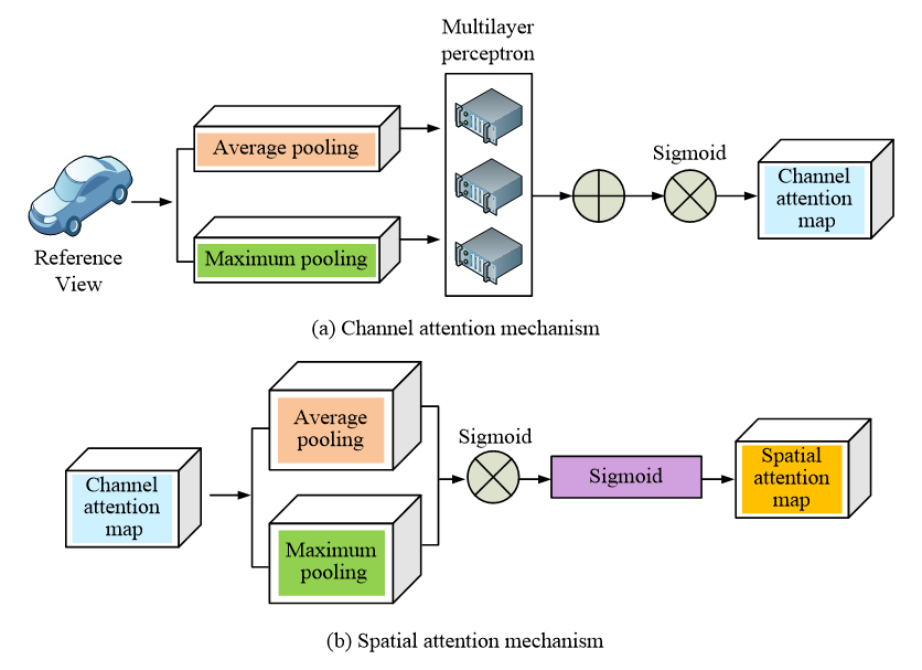
Fig. 5 Module diagram of CAM and SAM
Figure 5(a) shows the module diagram of CAM, and Figure 5(b) shows the module diagram of SAM. Each channel of the feature graph is treated as a feature finder, the essence of which is to model the importance between the various features, and the features assign inputs for different tasks. Therefore, the channel attention module expresses features more by inhibiting or enhancing different channels. For complex texture or diffuse reflection regions, a simple feature extraction network may cause some source view converted feature maps to lose details so that complete feature data cannot be obtained, and thus, the integrity of the reconstructed point cloud is reduced. Therefore, in the CAM module, Maximum and average pooling are employed together, and then feature city extraction is carried out by a shared weight neural network.
In the SAM, the spatial position of the sample points in the feature map is extremely important. If there is a deviation in the position, it will not be possible to ensure that the corresponding maximum probability point is the real point that originally existed in this space coordinate when selecting the probability. To highlight the information area effectively, the channel attention map is averaged and maximized along the channel axis, and then the spatial attention map is generated by the Sigmoid function. The equation for generating feature images is shown in Eq. (11):
(11)
In Equation (11), Ms represents the generated spatial attention map; F’i represents a feature map generated by SAM; F’i denotes the SAM feature map generated by maximizing pooling operations. σ is the activation function.
By combining the CBAM with MVSNet, the feature maps of each group of reference views and source views are more accurate after the homologous transformation. After the cost body aggregation, the original information is retained to the greatest extent to improve the integrity of the final reconstructed point cloud. Figure 6 illustrates the structure of the MVSNet feature network with CBAM.
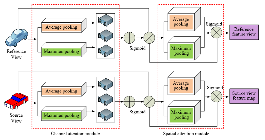
Fig. 6 MVSNet module diagram using CBAM
Figure 6 shows the MVSNet module diagram using the CBAM. First, the view graph of the scene to be reconstructed is traversed. For each image, it is input as a reference view along with its nearby source view. Then MVSNet is used to extract features from the reference view and source view, and the generated feature map is used for homologous transformation and bilinear interpolation. The CBAM is adopted in the last four layers of the MVSNet so that key feature information can be extracted and the relationship between features can be strengthened when the feature abstraction reaches a certain degree. The maximum and average pooling methods are applied to aggregate the feature information, and the generated bi-dimensional features are input into a shared weight network to obtain the channel attention diagram. The attention map is multiplied and added with the input image, and then the channel attention map is maximized and average pooled successively. Then, the required weight graph is generated by the Sigmoid function. The input channel attention diagram is used to multiply and add the appropriate components. The obtained spatial attention diagram is used as the final feature map.
4. Performance verification of MVSNet-CBAM model
To reduce the systematic error of the experiment, the performance test of the algorithm model was carried out in the same experimental environment. Table 1 demonstrates the experimental environment of the study.
Table 1 Experimental environment information
| Name | Configuration |
| Video card | NVIDIA GTX1080Ti |
| CPU | I7-8700K |
| Gpu-accelerated library | CUDA 10.0 |
| Memory | 16 GB |
| Operating system | Ubuntu16.04 |
| Algorithm framework | Pytorch |
To verify the validity of the research method, MVSNet, Multiple View Stereo Network-Spatial Attention Mechanism (MVSNet-SAM), Multiple View Stereo Network-Channel Attention Mechanism (MVSNet-CAM), and Multiple View Stereo Network-Convolutional Block Attention Module (MVSNet-CBAM) models were selected for experimental comparison. The data sets used in the experiment are the classical data sets of MVS, including DTU, ETH3D, and BlendedMVS. Firstly, four different models were trained. Figure 7 illustrates the loss function curve.
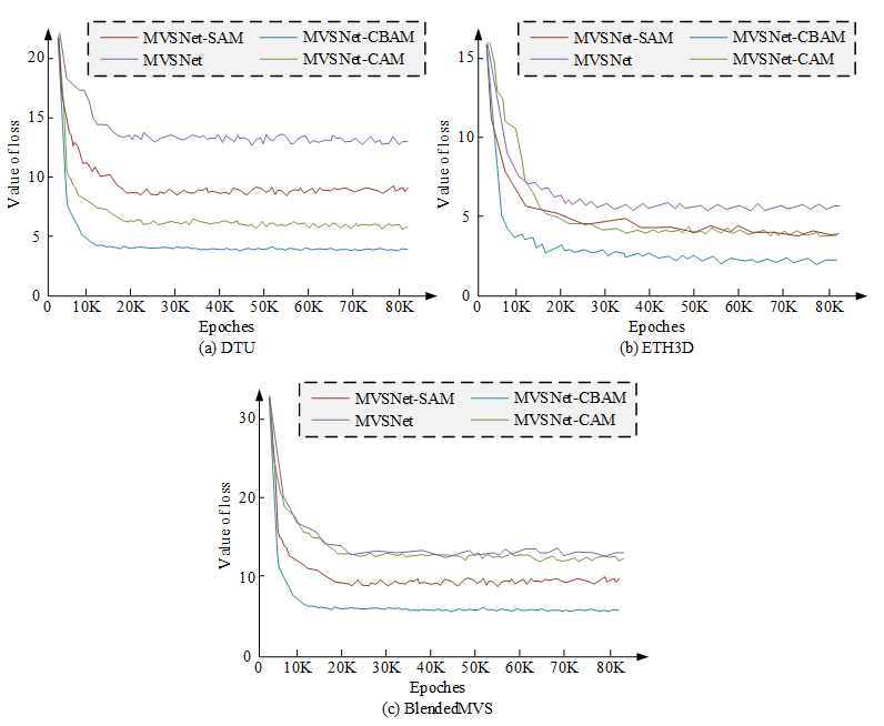
Fig. 7 Loss function curve
Figure 7 displays each model’s loss function curve in the DTU data set. The lower the loss function is, the better the model fits. Figure 7 (a) shows the loss function curve of each model in the DTU data set. In the figure, MVSNet-CBAM shows the most obvious downward trend. At steady state, the loss function value of MVSNet-CBAM is the lowest, about 4, which is reduced by 71.42%, 51.81% and 44.29% compared with the other three models, respectively, indicating that MVSNet-CBAM has the best fitting. In addition, MVSNet-CBAM has the least number of iterations when it reaches stability and approaches convergence around 10K, indicating that the model has higher computational efficiency and accurate results can be obtained quickly. Figure 7 (b) displays each model’s loss function curve in the ETH3D data set. In the figure, after the 30K iteration, the loss function curves of each model have nearly converged. When steady, the loss function value of MVSNet-CBAM is the lowest, about 3, which is reduced by 59.24%, 45.24% and 44.21%, respectively, compared with the other three models. MVSNet-CBAM is also close to converging at around 10K. Figure 7 (c) displays each model’s loss function curve in the BlendedMVS data set. In the figure, after the 20K iteration, the loss function curves of each model have nearly converged. After the loss function value is stable, the loss function value of MVSNet-CBAM is the lowest, about 6, which is reduced by 55.22%, 53.12% and 27.67% compared with the other three models, respectively. MVSNet-CBAM is also close to converging at around 10K. The training results demonstrate that this study’s model owns quicker convergence speed, lower loss function value, and better performance. After the training, the above four models were used for testing, and the research statistics were collected in the test of different data sets.
Table 2 Data of various evaluation indicators under different datasets
As shown in Table 2, the model evaluation indicators selected in the study include accuracy, integrity and comprehensive score. The higher the precision and the greater the integrity, the better. The overall score is the average of accuracy and point cloud integrity. The higher the overall score, the better. Overall, the accuracy was ranked from best to worst, namely MVSNet-CBAM, MVSNet-CAM, MVSNet-SAM, and MVSNet. In terms of integrity, they are ranked from best to worst, namely MVSNet-CBAM, MVSNet-CAM, MVSNet-SAM, and MVSNet. In the overall score, MVSNet-CBAM, MVSNet-CAM, MVSNet-SAM, and MVSNet were ranked in order from best to worst. The statistical results illustrate that MVSNet-CBAM has the best performance, which verifies the validity of this study. Verify the suggested model's performance using various indices. The accuracy test results were obtained, as shown in Figure 8.
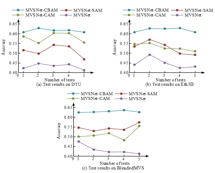
Fig. 8 Test results of accuracy
Figure 8 shows the test results of accuracy in the DTU data set, and the higher the accuracy, the better the model. MVSNet-CBAM has the highest accuracy, followed by MVSNet-CAM, then MVSNet-SAM, and finally MVSNet. Compared with the other three models, the accuracy of MVSNet-CBAM is improved by 17%, 9% and 3%, respectively. Figure 8 (b) shows the test results in the ETH3D dataset. MVSNet-CBAM has the highest accuracy, followed by MVSNet-CAM and MVSNet-SAM, and MVSNet has the lowest accuracy. Compared with the other three models, the accuracy of MVSNet-CBAM is improved by 15%, 4% and 4%, respectively. Figure 8 (c) shows the test results in the BlendedMVS dataset. MVSNet-CBAM has the highest accuracy, followed by MVSNet-SAM, then MVSNet-CAM, and finally MVSNet. Compared with the other three models, the accuracy of MVSNet-CBAM is enhanced by 20%, 13% and 9%, respectively. It is verified that the accuracy of MVSNet-CBAM is the best among the models involved in the comparison. Further test the integrity performance, as shown in Figure 9.
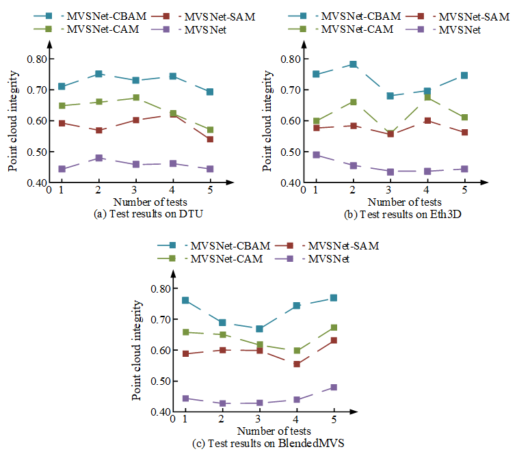
Fig. 9 Test results of point cloud integrity
Figure 9 shows the test results of point cloud integrity in the DTU data set. The higher the point cloud integrity, the better the model. The integrity of MVSNet-CBAM is the highest, the integrity of MVSNet-CAM is similar to that of MVSNet-SAM, and the integrity of MVSNet is the lowest. Compared to the other three models, the integrity of MVSNet-CBAM was enhanced by 28%, 14% and 9%, respectively. Figure 9 (b) shows the test results in the Eth3D dataset. The integrity of MVSNet-CBAM is the highest, the integrity of MVSNet-CAM and MVSNet-SAM is similar, and the integrity of MVSNet is the lowest. The integrity of MVSNet-CBAM was enhanced by 27%, 14% and 10%, respectively, compared to the other three models. Figure 9 (c) shows the test results in the BlendedMVS dataset. MVSNet-CBAM has the highest integrity, and MVSNet has the lowest integrity. Compared with the other three models, the integrity of MVSNet-CBAM was enhanced by 31%, 16% and 14%, respectively. It is verified that the model can reduce the integrity error of image construction. The comprehensive scores of each model were compared, as shown in Figure 10.
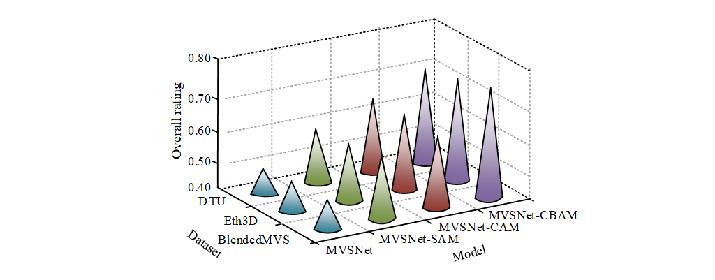
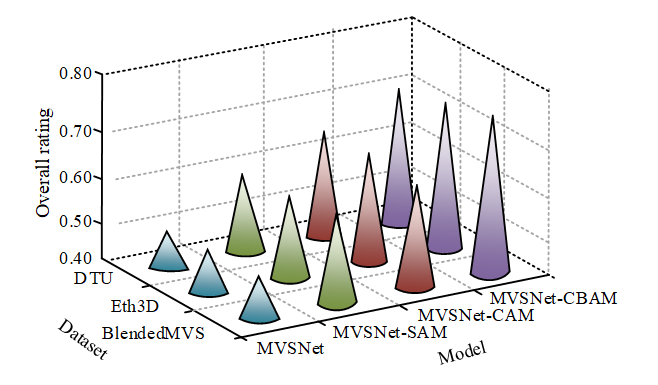
Fig. 10 Results of the overall rating
In Figure 10, the MVSNet-CBAM model proposed in the study has the highest comprehensive score, which proves that the model is the best. MVSNet-CAM is similar to MVSNet-SAM, but both are superior to the traditional MVSNet model, which confirms the efficacy of the CBAM optimization in this investigation. In addition, the results of different data sets also reflect that this study’s model has good stability.
5. Conclusion
3D digital image virtual scene reconstruction algorithm is a popular research direction of computer vision. With the 3D digital image virtual scene reconstruction algorithm, the real world can be restored with high precision and thus provide a new possibility for computer vision. In the current research, there is room for improvement in the accuracy and completeness of virtual scene reconstruction. Therefore, based on the traditional 3D reconstruction algorithm, the multi-view stereo vision algorithm and neural network are used for optimization. The CBAM is used in the multi-view stereo vision algorithm model. In model training, MVSNet-CBAM has the lowest loss function value, reduced by 71.42%, 51.81% and 44.29% compared with MVSNet-CAM, MVSNet-SAM and MVSNet, respectively. In the test, the MVSNet-CBAM model proposed by the research has the highest comprehensive score, which proves that this model is the best. Although this study has achieved certain results, due to the limited experimental conditions, this study did not conduct a large sample experiment. Therefore, the research results are of reference value only. How to further improve the applicability of the research will become the main research direction in the future.
