
INTRODUCTION
The quest for quality of life is the ultimate goal for individuals and societies across the globe. Individuals’ assessment on the quality of their life in a country is of paramount significance for decision makers endorsing multifarious public policies. Basically, in a country striving for the betterment of the lives of its nations, while formulating public policies, analysts consider the potential impact of policies on the quality of citizens’ life patterns. Accordingly, some governments provide social services in an effort to strike a reasonable balance between the well-being of individuals’ and societies.
Though GDP per capita is the most commonly applied method of measuring the impact of economic activities and distribution of resources of a nation, it is criticized for being a poor indicator of a nation’s well-being[1, 2]. Initiatives featuring subjective ways of measuring well-being in a nation have recently gained momentum. Thus, the use of subjective well-being (SWB) indicators is recommended as they provide indispensable information. Well-being by its very nature is subjective and hence the SWB approach is based on the belief that a person cannot assess another person’s satisfaction with something in a country based on subjective parameters as opposed to objective criteria involving the person whose satisfaction is explored. In the SWB approach which treats a person as an authority, the researcher is, therefore, advised to focus on understanding the well-being from the view point of individuals under investigation[3].
Scholars have been writing on the role of welfare state on health[4], marital stability[5], family structure[6], gender equality[7], poverty[8, 9, economic growth[10], income inequality[11, 12], and SWB[13-16].
Of great interest in this article is the role of welfare state on SWB. In the SWB literature, studies on the link between welfare state and SWB have conflicting conclusions. Outcomes of studies of the relationship between welfare state and SWB are often messy. While decommodification[16], health care expenditures[15], and benefit replacement rates[13] have positive effects on individual-level self-rated well-being, social expenditure has no effect on aggregate SWB[14].
Some the studies consist of methodological problems. For instance, Veenhoven’s[14], analysis is predominantly based on bivariate correlations and it does not allow researcher to control for very specific issues. Moreover, Veenhoven’s[14] reliance on aggregate level data is problematic to analyse life satisfaction which is basically an individual-level and subjective experience. This tendency is at risk of making ecological fallacy with an improper hypothesis assuming that relationships at the aggregate-level may also hold at the individual-level devoid of objective parameters. Though[13] and Pacek and Radcliff[16] made an attempt to assess the effect of welfare state on individual-level SWB, their analyses put micro and macro variables together without considering the hierarchical nature of the variables. Given the fact that individual-level SWB is determined by the combination of both country-level characteristics and individual-level factors, multi-level analysis can be considered appropriate. Bonini[17], for instance, argues that 19 % of variations in individual-level SWB are explained in terms of country-level differences.
The main objective of this article is, therefore, to assess the extent to which welfare states make their citizens satisfied (happy) with everything they need in their respective countries, while keeping individual-level variations constant. In order to minimize the potential problem of ecological fallacy, the article analyses the nexus (connection) between welfare state and individual-level SWB without changing their multi-level nature. Hence, the article centres on two concepts: subjective well-being and the welfare state.
SUBJECTIVE WELL-BEING AND THE WELFARE STATE
SUBJECTIVE WELL-BEING
Subjective well-being can be defined as people’s evaluation of the quality of their own life as a whole[18]. The study of SWB is often features a survey research that enquires perceived level of satisfaction of individuals[19, 20]. In SWB (wellbeing) literature, there is a clear distinction between affective SWB and cognitive SWB[21].
The affective component of SWB, reflects the balance between pleasant and unpleasant feelings in people’s lives (i.e. happiness, joy). Affective theories maintain that “happiness is a reflection of how well [individuals] feel generally”[22]. This component of SWB is associated with people’s moods and feelings. Affective component of SWB is divided in to two, i.e. positive and negative instances of affective well-being. They are usually measured by asking people how often they felt happy, angry or depressed[18].
The cognitive component of SWB, reflects individuals’ evaluations of their lives (i.e. life satisfaction, satisfaction with domains of life).Cognitive theories indicate that “happiness is a product of human thinking and reflects discrepancies between perceptions of life-as-it-is and notions of how-life-should-be” Veenhoven[22]. In other words, the cognitive component of SWB refers to people’s assessment of how satisfied or dissatisfied they are with their lives. Satisfaction with life is a bottom up approach which is a sum of feelings and the satisfaction with different domains of one’s life. According to Veenhoven[23], satisfaction with life has four components: pleasure (part of life passing satisfaction), part-satisfaction (part of life enduring satisfaction), top-experience (life-as-a-whole passing satisfaction), and life-satisfaction (life-as-a-whole enduring satisfaction). For the sake of convenience, in this article, subjective well-being and life-satisfaction have been used interchangeably.
THE WELFARE STATE
The term welfare state is differently viewed by different scholars. Each variety of views has different public policy implications[24]. According to Briggs[25],a welfare state is “a state in which organized power is deliberately used (through politics and administration) in an effort to modify the play of market forces in at least three directions”. Such modifications can happen by offering minimum income regardless of market values of citizens, preventing citizens from “social contingencies”, and offering social services without discrimination. Even though all states have “the right and duty” to work for the betterment of their citizens[26], welfare states are those that actually provide services to benefit their nationals.
Welfare state measurement approaches can be summarised as the expenditure approach and entitlements approach even though different methods can be applied to measure differences in welfare states. The former measures actual government spending. This indicates the size of welfare state. It can be measured by calculating the extent to which countries spend resources on social policies (an aggregated spending on several different groupings of social programs) as compared to their GDP. Given that there are differences in conceptual definitions of social policy programs across countries, comparing welfare states on the basis of data about social spending is often problematic[27]. However, the latter approach shows the legal rights of the public for benefits. This approach assesses the degree of generosity of social policies in the country (e.g. pension replacement rate, unemployment replacement rate, etc).
Globally, welfare states are dissimilar. Esping-Andersen’s[28] “the three worlds of welfare capitalism” was the first to cluster welfare states into three families – liberal, conservative, and social democratic – based on decommodification, social stratification, and the private-public mix. In brief, the liberal welfare state is closely related to traditional work-ethic norms
“in which means-tested assistance, modest universal transfers, or modest social-insurance plans predominate”[28]. Conservative welfare states (e.g. Germany) are committed to provide welfare services but the issue of preserving social status differences is strong. Moreover, the role of churches and families in delivering social services is very strong. In this type of welfare state, the male bread winner family tradition is kept alive. In social-democratic welfare states “universalism and decommodification of social rights are extended to the new middle classes”[28]. This regime advocates social equality in order to achieve utmost standard through full participation of workers.
Esping-Andersen’s[28] the Three Worlds has become a footprint in exploring the specifics about welfare regimes[29,30]. In this regard, Ferrera[31], Korpi and Palme[12], propose alternatives to Esping-Andersen’s[28] classification. Alternatives to Esping-Andersen’s[28] typology show that though some welfare states consistently fit in one category, many others may not do so. This is mainly because welfare typologies change depending on the criteria and time. For instance, the Dutch welfare state shows a shift form Corporatist in the 1960s, 1970s and early 1980s to Social Democratic after the 1980s[32]. Esping-Andersen’s[28] regime types have been criticised for being limited in reflecting the situation in different parts of the world (i.e. Mediterranean, Central and Eastern European, Asian countries, etc). Fenger[33], for instance, argues that Central and Eastern Europe should be grouped separately as “the level of trust, the level of social programmes and social situation in the post-communist countries are considerably lower than [their counterparts] in the other countries”.
Though many of the studies on welfare state typologies focus on few advanced countries, Abu Sharkh and Gough[34] managed to generate clusters of welfare states out of OECD. Cluster A, Abu Sharkh and Gough state, is about a group of countries that show some characteristics of western welfare states such as extensive state commitments to welfare provision, relatively effective delivery of services and moderately extensive social and superior welfare outcomes security programmes. In cluster B, countries with combination of low social spending and low dependence on aid and remittance from abroad are clustered. In cluster C, there are countries with great dependence on external flow of remittance. Cluster D is characterised by relatively extensive public social programs, moderately good welfare impacts and high literacy but with very low life expectancy. Although with high levels of youth literacy, Cluster E comprises a group of countries with fairly high foreign aid reliance and low rates of girl literacy. In Cluster F, though there is high expenditure on social programmes and informal security mechanisms, there are high levels of insecurity and illiteracy. Clusters G and H are composed of weak states that are highly dependent on foreign aid with low level of public responsibility and life expectancy.
As noted above, the concern of this article is with the association of welfare state on SWB. In a study on aggregate-level data, Veenhoven[14] found “no connection between the size of state welfare and equality in well-being between its citizens. In countries where social security expenditure is high, the dispersion of health and happiness is not smaller than [that of] equally prosperous countries with less public sector spending”. This study employs simple correlation analysis which does not allow the researcher to control for variables that could possibly affect SWB. Kotakorpi and Laamanen[15], on the other hand, reported positive relationship between relative expenditures on social services and SWB of the average citizen in Finland.
Furthermore, Di Tella, MacCulloch[13] disclosed that benefits replacement can have positive effect on SWB. Similarly, Pacek and Radcliff[16] argued that “welfare state generosity exerts a positive and significant impact on life-satisfaction and happiness”. Though these studies employed sophisticated methods, they failed to maintain the multi-level nature of SWB and welfare state.
In nested data structure, traditional regressions may lead to false conclusions. When data are clustered, single-level regression analyses are not suitable since the fundamental premise of independence of the observations is violated. Because of this, standard errors estimated in single-level regression are small resulting “many spuriously significant results”[35]. As Snijders and Bosker[36] put it: “For the data with meaningful multilevel structure, it is practically always unfounded to make the a priori assumption that all of the group structure is represented by explanatory variables. [...] In designs with group sizes larger than 1, [...] the nesting structure often cannot be represented completely in the regression model by the explanatory variables. Additional effects of the nesting structure can be represented by letting the regression coefficients vary from group to group.”
To model between country differences, it is, therefore, important to allow the intercept vary between countries. The presence of conflicting results and methodological limitations on previous studies beg for further investigation. Based on the literature review, this article hypothesizes that:
H1: most of the proportion of variability on SWB could be attributed to country level differences,
H2: differences in welfare regime typology contribute to variations in individual-level SWB,
H3: iindividual’s SWB would differentiate based on public social spending,
H4: generosity of welfare state would have positive effect on individual’s SWB.
DATA AND METHODS
THE DATA
The data for all individual-level variables used in this research were obtained from the sixth wave (2010-2014) of the cross-national World Value Survey[37]. The sixth wave of the WVS was used because of the presence of a richer mix of countries which is important to get a better degree of variation across countries. The WVS is a very useful source of data that can be used to analyse cross-national differences in social attitudes and values globally. With regard to sampling, simple random samples based on the population of each of the participating nations was employed regardless of nationality, citizenship or legal status. The data for a country level variables were taken from International labour Organization[38] (ILO) and Organisation for Economic Co-operation and Development (OECD).
This article presents an analysis on the data from 20 countries (N = 33879). The countries included in the analysis are Australia (n = 1010), Brazil(n=1434), Chile (n = 876), China (n = 1961), Estonia (n = 1497), Germany (n = 1928), India (n = 4986), Japan (n = 1765), Korea (n = 1138), Mexico (n = 1919), the Netherlands (n = 1578), New Zealand (n = 681), Poland (n = 908), Russia (n = 2 236), Slovenia (n = 978), South Africa (n = 3 216), Spain (n = 1022), Sweden (n = 1108), Turkey (n = 1513), and the United States (n = 2 125).
VARIABLES
The dependent variable is individual-level SWB. As discussed earlier, life satisfaction measures how people assess their life as a whole rather than their individual present feelings. Previous studies were focused on the cognitive component of SWB arguing that life satisfaction item is a more reliable indicator. Accordingly, life satisfaction item was selected as a measure of SWB. On a scale from 1 to 10, the WVS presented the following question to respondents: “All things considered, how satisfied are you with your life now?”
Welfare state typology is one of the independent variables of interest. Even though there are different welfare regime typologies, in this study, countries are grouped based on the consistency of categorization in previous studies (see[29,30] for the details). Basically, welfare regimes in European/OECD countries are categorised as social democratic (Sweden and the Netherlands), conservative (Germany, Spain), liberal (Australia, Japan, New Zealand, and the United States), and central and eastern Europe (Estonia, Poland, Slovenia and Russia). Countries out of OECD are categorised based on Abu Sharkh and Gough[34] as cluster A (Brazil), cluster B (Chile, China, Korea, and Mexico), cluster D (South Africa), and cluster F (India). In order to assess the different effects of welfare regimes at an individual level well-being, a dummy-variable for each welfare typology is created.
Welfare entitlement is also one of the variables of particular interest in this article. According to the Organisation for Economic Co-operation and Development[39], the net pension replacement rate is defined as “the individual net pension entitlement divided by net pre-retirement earnings, taking account of personal income taxes and social security contributions paid by workers and pensioners”. Net pension replacement rate of sampled countries for 2014 collected from the Organisation for Economic Co-operation and Development[40]was employed. The indicator used to measure the size of welfare states is total public social expenditure as percentage of GDP reported by the International labour Organization[38] in its Social Security Inquiry (SSI).
Moreover, to understand the role of welfare state in individuals’ SWB controlling individual-level variations is vital. Accordingly, a wide range of factors attributed to a specific person, such as gender[41], age[42], marital status[43], education level[44], health status[20], income[45, 46], employment status[47], and religion attendance[48] are controlled.
THE METHOD
The data used are cross-sectional and without rooms for cause-effect analysis. That is, the establishment of temporal order is crucial for a causal data interpretation. This article, therefore, focuses on identifying the association between welfare state and individual-level SWB, thereby keeping personal characteristics constant.
This study involves a special kind of regression, i.e. multi-level mixed-effect linear modelling. Applying multi-level modelling is practical to assess the effects of individual and country-level variables at an individual-level SWB. This kind of analysis is indispensable for explaining how much of the variation in the level of SWB can be explained in terms of contextual and personal characteristics considering the nested structure of data.
Multi-level models, also known as hierarchical models or Mixed-effects models, consist of both fixed (estimated directly) and random effects (not directly estimated). For continuous responses multi-level models are linear regressions that include random effects in addition to variations linked to the error term. In situations where the data is clustered and individuals are grouped in each country, it is appropriate to arrange the mixed model as a series of independent clusters. Applying Ordinary Least Square (OLS) regression analysis by considering all observations together, in this case, is problematic. First, estimates tend to be wrong as standard errors produced cannot be trusted. Second, OLS regressions do not show extent of variation explained at a country-level and an individual-level. In other words, such method of analysis does not explain the degree to which country-level variations affect individuals’ SWB after controlling individual differences.
Accordingly, in order to obtain the estimates through a mixed method, an application that uses residual maximum likelihood (REML) estimation procedure[49], which is appropriate for smaller cases at the second level was applied. REML regressions yield unbiased estimates of parameters[50].
In the random intercept model, the intercepts β0j are random variables representing random differences between groups[50]:
where Yij is a dependent variable, i is a level-one unit, j a level-two unit, xij the explanatory variable at level-one for group j, Zj explanatory variable at level-two, nj groupsize, β0j are intercepts, β1 the coefficient for level-one variable and β2 the coefficient for level-two variable.
The intercept is the summation of average intercept (γ00) plus group-dependent deviation (U0j):
In random intercept model, the regression coefficient β1 is common to all the groups. In the random intercept model, the constant regression coefficients β1 and β2 are sometimes denoted asγ10and γ01 respectively.
Substitution yields:
In this article, fixed effects of explanatory variables are included. In the multi-level model, the U0j signals random variables. The model assumes that they are independent, i.e. normally distributed. Their variance is: τ2 = var(U0j).
The empty model, that is, the model with no explanatory variables can be written as:
In this model, the total variation in the dependent variable is divided between individual variation and variance at a country level. U0j represents individual variation in a given country (level-two), while Rij is variation attributed to country level differences (level-two). Variance decomposition is:
Covariance between two individuals i and i’ (with i ≠ i’) in the same group j is obtained as follows:
Intra-class correlation (ICC) is coefficient that gives information on the proportion of variability that can be attributed to level-two. It can be defined as the ratio between country variance and the total variance. The ICC show the data in the group, i.e., the smaller the ICC, the lesser the data are clustered. ICC is as follows:
Multi-level mixed-effect linear model of the subjective well-being equation can be outlined as:
with SWBij denoting the dependent variable, i individual level, j country level, xij individual-level explanatory variables for each country; Zj country-level explanatory variables, γ00 intercept, γ10 coefficient for individual-level variables, γ01 coefficient for country-level variable, U0j country-level residuals and Rij individual-level residuals.
RESULTS AND DISCUSSIONS
Using the data at individual and country-levels, this article analyses the association between welfare state and SWB. Before investigating the effect of welfare state on individual-level SWB using multi-level models, it is better to examine their macro-macro relationships. Table 1 shows Pearson correlation coefficients.
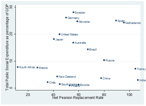
Table1 indicates that there is no correlation between size of welfare state (social expenditure) and welfare generosity (net pension replacement rate). Moreover, the scatter plot shows that the sampled countries are with different degrees of generosity and dissimilar sizes of economic welfare state (see Fig. 1). Social expenditure as percentage of GDP ranged from 1,0 (in Poland) to 28,13 (in Sweden), averaging 11,85. This indicates that there is a wide gap in social expenditure as percentage of GDP. The average net pension replacement rate is 61,42 %: ranging from 11,8 % to 106,75 %.
Out of the sampled countries, India and South Africa are the most generous and the least generous countries respectively. As can be observed in Figure 1, in terms of net pension replacement rate, India ranked the most generous state, whereas in terms of public social expenditure, India is among the least spenders. This indicates that spending more on social services does not necessarily mean that the country spends all the money on social programs. That is, generosity and social expenditure do not yield the same result.
In Figures 2 and 3, country-level average life satisfaction and welfare state indicators (size and generosity) are mapped out respectively. Average life satisfaction scores in all of the countries under investigation appear to be tilted towards the highest possible response. The
Net Pension Replacement Rate
average country-level life satisfaction ranged from 6,05 to 7,86 with an average of 7,09. On average, Brazilians are the most satisfied people with life and Indians rate themselves as the least satisfied.Based on the result of the bivariate correlation analysis, there is statistically significant relationship between social expenditure and average life satisfaction (Table 1). Moreover, some countries (Germany, the Netherlands, Slovenia and Sweden) which spend much on social programs reported higher level of SWB (cf. Figure 2). Average life satisfaction of people living in countries that spend few on social programs (Estonia and India) is very low. However, SWB in Switzerland and New Zealand is high even though they spend somehow lesser on social services.
Concerning welfare entitlement, on the one hand, people living in countries (Netherlands and Turkey) with higher net pension replacement rate enjoyed higher average SWB. On the other hand, average SWB is low in India and Russia, even if there is high replacement rate. The correlation analysis, therefore, shows that there is no correlation between net pension replacement rate and average SWB (Table 1). Such contradicting outcomes need further analysis in relation to the interplay between individual factors and national context in affecting an individual-level SWB. The next sections deal with such relationships. Consequently results of multi-level mixed-effect linear regression analysis are presented.
Table 2 summarises results of multi-level mixed-effect linear models. The empty model without explanatory variables is presented as baseline. Model 1 contains both individual and country-level variables. This model explains the effects of size and generosity of welfare state at an individual-level SWB while keeping potentially useful predictor individual-level variables constant. To check whether or not there is log linear relationship between welfare state and SWB; logarithm functions of size and generosity of welfare state have been included in model 2. Model 3 contains welfare state regimes. Finally, in model 4, the combination of model 1 and 3 has been provided.
The dependent variable in all models is life satisfaction. In Table 2, the reference dummy is in square brackets and Standard Errors in parenthesis. Abbreviations in Table 2 are as follows: NPPR – Net Pension Replacement Rate, TPSE – Total Public Social Expenditure (as a percentage of GDP), SD – Social Democrat, CEE – Central and Eastern Europe[37].
Before starting to investigate each coefficient, one needs to assess how fit the models are. In selecting the model that best fits, looking at the values of Akaike information criterion (AIC) and Bayesian information criterion (BIC) is vital. Such a model is the one with the smallest AIC and BIC values. In cases where the two criteria yield different results, the AIC takes precedence[51]. In this case, all the models are statistically significant. The information about models that best fit indicates that the models with coefficients are much better than the empty model. Moreover, model 3 is the best fitting model with the lowest AIC value.
On the basis of the multi-level mixed-effect method of analysis, the variance in each level is examined. Concerning the first hypothesis, this article revealed an intra-class correlation (ICC) of 0,08 (Table 2). Contrary to the hypothesis, small portion of the variation in an individual-level SWB can be explained by country-level variations. That is, only 8 percent of the variation in individual-level SWB is explained by country-level variables. This indicates that an individual-level SWB ratings, though to smaller extent, are affected by national contexts. ICC values between 0,15 and 0,25 are common in social science studies [36, 52]. At this juncture, it would be useful to test out whether or not a welfare state is responsible for variations in an individual-level SWB.
The relationship among impacts of different welfare regimes on an individual-level well-being across the globe has been explored. There is no significant difference in an individual-level SWB among European/OECD welfare regimes (i.e. social democrats, liberal, and conservative). SWB of individuals living in most of the welfare regimes outside of OECD is significantly different from that of European/OECD welfare regimes. While people living in cluster A reported significantly higher level of SWB, those in cluster D and F reported the opposite.
*significant at 5 % probability level
**significant at 1 % probability level
***significant at 0,1 % probability level
This can be associated with the growth-to-limits syndrome as any European/OECD welfare state has already reached its maximum level. of coverage and generosity. For instance, almost all Europeans are eligible for “social protection schemes for all the ‘standard risks’: old age, disability, and bereavement; sickness, mentality, and work injuries; unemployment and family dependants”[53]. In such cases, welfare classifications may not significantly contribute to the variation in well-being. However, European/OECD and non-OECD welfare regimes are very different in nature. Such differences contribute to the difference in individual-level SWB.
Concerning the third and fourth hypothesis, after individual characteristics were analyzed, it was found that there was neither linear nor log-linear relationship between welfare state and an individual-level SWB (cf. model 1 and 2). That is, at any particular point in time, a respondent’s life satisfaction does not vary in size and generosity welfare state of a country. Thus, at a particular time, variation in welfare spending as well as welfare entitlements across countries does not have a significant effect on SWB of citizens. In other words, though there are differences in size and generosity of welfare state, such differences do not generate considerable effects on SWB of individuals.
Moreover, this article argues that neither size nor generosity of welfare state has a significant effect on individual-level SWB. Different arguments are brought into the discussion about the relationship between welfare state and SWB. Partly, it is associated with the view of welfare state intervention with respect to taxation considering the fact that public social spending is financed by taxes collected from citizens. From the rational choice theory perspective, human beings as utility maximizing individuals may prefer to pay lower taxes. Hence, they would be unhappy with government spending and public social spending might decrease individual’s SWB. On the other hand, as for advocates of big governments, people may tend to pay higher taxes to consume much of public goods and ultimately live better lives. Moreover, given the decreasing marginal utility of income, redistribution from the rich to the poor may generate more SWB for both the poor and the rich[54].
Spending a good deal of resources on social programs may not necessarily affect all citizens in the same way. Individuals. benefiting from social welfare may have higher SWB as they are positively affected by such policies. Besides, the majority (in a society) do not yet enjoy the benefits of social welfare programs.
Another possible explanation is that a welfare state can have a negative effect on individuals’ well-being. According to Murray[55], spending more money on social programs designed to assist the poor and underprivileged tend to make things worse. Critics of welfare state claim that having a generous welfare state may encourage intentional unemployment. This can result in lower satisfaction of citizens as unemployment is an important determinant of SWB. Studies indicate that there is a positive association between the rate of unemployment in a region and the average loss of well-being[47]. Unemployment rate affects both employed and unemployed citizens. For unemployed people, unemployment rate negatively affects their well-being because of lack of income and socio-economic and psychosocial challenges. Moreover, even employed people tend to be unhappy about a low employment rate due to the potential negative impact of unemployment on their life patterns[13].
There are also financial and institutional constraints, such as mounting public debts and deficits, considering entitlements as property rights[56], and loss of SWB for individuals with the constraints Moreover, with regard to relevance of policies, the findings indicate that welfare states would neither increase nor decrease an individual-level SWB.
Finally, Table 3 compares results of single-level (OLS) and multi-level models. It can be noted that all of the welfare variables are significant in the single-level analysis. However, size and generosity of welfare, most noticeably, lose their significance in the multi-level model. Controlling for contextual differences variations, size and generosity of welfare state by themselves played less of a role in explaining individual-level SWB. As Hox[35] suggested, the significant effect found on OLS regression may be due to spurious effect. The multi-level model provides better estimation by revealing spurious nature of the relationship.
The dependent variable in all models is life satisfaction. In Table 2, the reference dummy is in square brackets and Standard Errors in parenthesis. Abbreviations in Table 2 are as follows: NPPR – Net Pension Replacement Rate, TPSE – Total Public Social Expenditure (as a percentage of GDP), SD – Social Democrat, CEE – Central and Eastern Europe[37].
*significant at 5 % probability level
**significant at 1 % probability level
***significant at 0,1 % probability level
CONCLUSIONS
This article presents analyses on the relationship between welfare states. and SWB in 20 countries (selected through purposive sampling) drawing on the WVS round 6 data. Previous studies dealt with mainly macro-macro relationship between welfare state and SWB, but this study employs multi-level analysis so as to investigate micro and macro level determinants of SWB. In this study, several interesting findings have been figured out.
The article argues that individual characteristics explain a large portion of the variation within individual-level SWB. The proportion of variance in individuals’ perceived SWB .has been left for further scrutiny in terms of country-level characteristics. This indicates that policy makers need to work on individual-level characteristics (such as individual-level income, employment, education, marital status, etc.) than country-level contexts in order to improve SWB of individuals.
The article also revealed that there is no significant difference in individual-level SWB among European/OECD welfare regimes. In relatively developed welfare states, the effect of
welfare typologies on individual level is insignificant. However, there is a visible difference in SWB between citizens living in and out of European/OECD welfare regimes.
Finally, as for Veenhoven[14] “[a] welfare state does not have to be kept intact at all costs”. It can be of great significance provided that it is suitable for nations employing it for their multifaceted development.