
1. INTRODUCTION
There are two interlinked essential arguments on tourism demand that underlie each other and together show the importance of the decisions of economic agents and geographical matters in how tourist flows are configured. In the first argument, the nature of tourism is examined in terms of how potential visitors who are located at a physical distance, where the consumption decision is made, make the decision to travel to enjoy their choice of a selected final destination (Swarbrooke and Horner 2007). The second argument examines the relative importance of geographic factors, given that countries have a natural-geographic endowment that is related in the future course of their spatial development (Venables 1998). In relation to flows of goods, financial resources and travelers, economic geography is undergoing reconsideration in studies and simulations at the regional level, with an awareness of the role played by geographical factors in the configuration of development patterns at the regional and national level (Yang et al. 2010). The consideration of traveler flows and relationships of economic geography is thus justifiable, as the present study will allow for a systematic examination of the strengths and weaknesses of regional, territorial units with respect to their attractiveness for visitors, which allows the invigoration of different economic enclaves of their production apparatuses. On this subject,Claveria et al. (2015) highlight the importance of the origin–destination distance as an explanatory variable that helps differentiate between groups of tourism.
At the international level,Vargas et al. (2007) andKeum (2010) have posited an analysis of tourist flows based on panel data models, finding significant variables that explain tourist behavior. However, such models have had few applications in the analysis of the behavior of these variables, particularly in terms of the use of the mixed linear model for these types of studies with data from Colombia (Vanegas et al. 2018). These models address the estimation from the multivariate theory, facilitating the inclusion of several countries in the estimation of a model to assess the determining factor and explain the variations of the tourist flows to a country. This multivariate approach has the advantage in that it considers the autocorrelations of the response variables, as other works have demonstrated, for example, for multivariate tourism forecasting (Claveria et al. 2015).
The travel and tourism industry encompasses significant economic activity in most countries, with direct and indirect incidences in productive apparatus (WTTC 2014). In this sense, forecasting process approaches and their relations with geographic and political attitudes or behavioral variables may be relevant in carrying out an appropriate planning resource to improve the economy of a region (Padhi and Pati 2017). This serves as a reason to search for more forms to increase the accuracy of forecasts, as some investigations demonstrate (Athanasopoulos et al. 2011;Chu 2014;Guizzardi and Mazzocchi 2010;Song et al. 2012).
Its contribution to the Colombian economy has exhibited some of the most dynamic behavior of any sector, with impactful contributions to employment and wealth generation. In the last 20 years, the dynamics of traveler flows as well as the expenditures associated with the destinations visited have showed sustained growth and significant financial contributions. Touristic movements of people and expenditures for travel items (dollars) have grown at an annual average rate of 8.2% and 46.7%, respectively, for 20 years between 1995 and 2014, although both slowed down somewhat during the 1999 Colombian banking crisis, but the trend was reverted to, and tourism recovered, reaching historical highs in the mid-2000s (Figure 1).
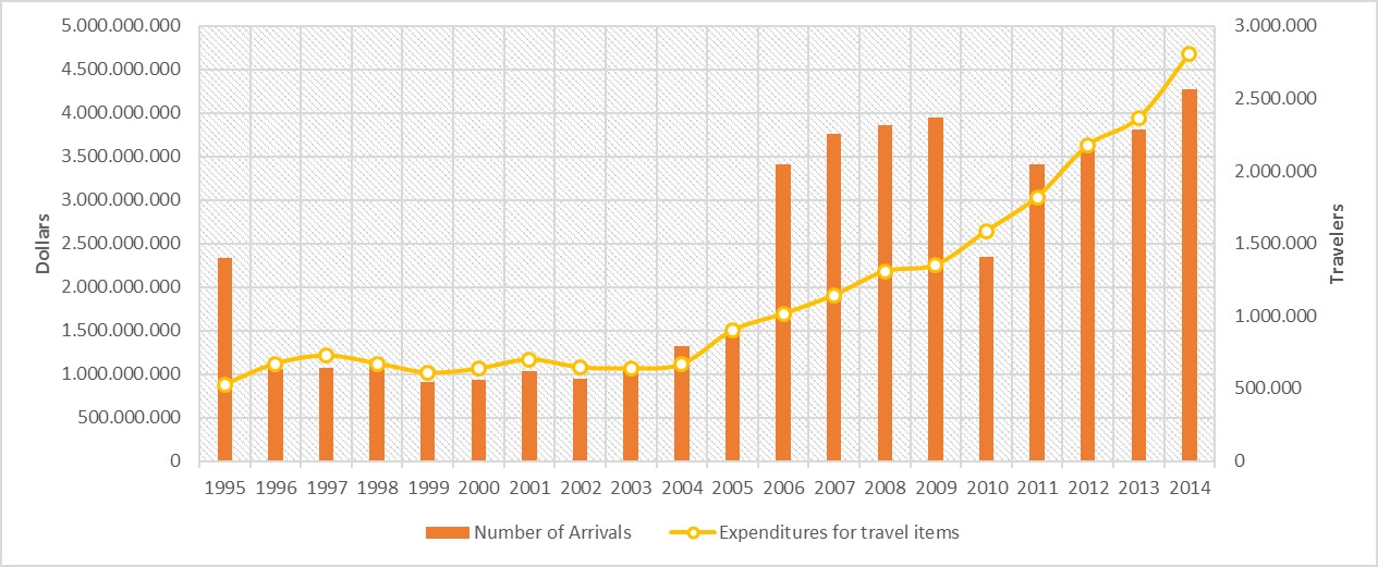
Source: own elaboration using data fromUNWTO (2016).
From a methodological point of view and by identifying explanatory factors and demand effects,Li et al. (2005) argued that the implementation of specialized econometric techniques allowed for a broader picture of international tourist flow behavior. By understanding the factors that determine the demand for tourism, public policies can be designed toward the creation of strategies that affect the development of tourism for countries. In particular, since 2010, tourist flows in Colombia have grown by 150%, from 2 million to 6.5 million (MinCIT 2018). In this sense, modeling tourism demand in countries with a promising sector growth may constitute an important aspect for improvement in order to achieve efficient profitability (Akın 2015).
Previous behavior contextualizes the importance of studying the main factors that explain tourist flows. This work estimates the determining factors attracting international tourists to Colombia, from the theoretical perspectives of both consumer behavior and the new economic geography, assessing the importance that these factors have in relation to tourism demand. This will help with decision making for economic agents, management decisions, marketing strategies, and planning improvements based on the impacts of geographic conditions and distances between countries over the tourist’s arrivals and on the linear mixed models’ analysis. Thus, the central questions are as follows: What are the main determinants of international tourism demand into Colombia? Are there spatial differences in the settings of traveler determination?
Tourism planning requires high investment levels on equipment, infrastructure, hotels, resorts, and staff training. These, in turn, require time horizons that fit both real and potential demand forecasting. Such strategic planning entails studies with advanced methods that serve the purpose of defining entrepreneurial goals in the fields of infrastructure, marketing, staff, and suppliers. Furthermore, these studies should also help predict the economic impacts derived from changes in the tourism market. Tourist flows into and out of Colombia have shown a surprising growth in the last few years, which tend to grow stronger at short- and mid-term intervals because of the implementation of the Colombian Peace Agreements. In spite of this, the literature that explores the determining factors within this topic is scarce, which is the reason that the present study expects to contribute to the field in the context of Colombia.
This manuscript is organized into five sections. Empirical studies concerning tourism demand are presented after the Introduction. The methodological approach is subsequently outlined, and the statistical techniques and sources of information are explained. The fourth section discusses the results, and conclusions are offered in the final section.
2. LITERATURE REVIEW
A central question in the determination of tourist flows focuses on the choice of destinations by travelers. An extensive number of works that estimate these flows on a country-by-country basis examine the determinants within the framework of partial or general equilibrium models, panel data, simultaneous equations, probabilistic models, and auto-regressive factors, among others (Su and Lin 2014;Ibrahim 2011;Massidda and Etzo 2012;Peng et al. 2015). Studies in this vein typically examine how exogenous macroeconomic factors affect tourist decisions, focusing primarily on incomes and movements in exchange rates. At the international level, the literature concerning world tourist flows, without specifying countries, is much broader, estimating global, continental, and national determinants. The literature exhibits a great variety of approaches for stimulating the determinants of the tourism demand of the world, a continent, or a country; within this, there are several factors that can be grouped into different areas such as economic, political, security-related, and geographical factors.
In the case of the application of gravity models,Morley et al. (2014) proposed a theoretical framework accounting for bilateral tourist flows based on the individual utility theory. The importance of this model in the estimation of tourism demand is highlighted, requiring a modeling of the role of structural factors in tourism.Morley et al.’s (2014) work demonstrated the difficulty of distinguishing the recent versions of gravity models and their suitability when discussing the structural factors to be assessed and quantified in relation to touristic demand. Other empirical studies that have focused on assessing the gravity determinants of tourism includeKeum (2010),Deluna and Jeon (2014),Kaplan and Aktas (2016), andTavares and Leitão (2017).
Few works have addressed the case of Colombia.Bonilla and Moreno (2010) studied the effects of security and trade; using a panel data model, they found that the arrival of foreign travelers was inversely related with kidnappings and commercial exchange indices were conducted in a positive manner. Other works have examined the local dynamics of the movements of travelers.Cerda and Leguizamón (2005), using hedonic models, found that the internal demand for national actors for the consumption of tourism products depended greatly on the profile of the head of household, household purchasing power, and household composition. In municipalities or at specific locations, for example, in the case of Cartagena, researchers have observed the impact of fluctuations in the exchange rate on tourism demand (Galvis and Aguilera 1999). Finally, classical and Bayesian regression models have been used in the estimation of the tourism demand for the city of Medellín (Valencia et al. 2017), andVanegas et al. (2018) compared different models for the estimation of tourist flows to Colombia.
There is a growing body of literature on work at the country level.Garin-Munoz and Amaral (2000) estimated that incomes, prices, exchange rates, and the Gulf War were all significant for explaining international tourist flows to Spain. For the African continent as a whole, the results ofNaudé and Saayman (2005) suggested that the arrival of travelers depends on the political stability, tourism infrastructure, marketing and information, and the level of development in the destination. For the case of Egypt,Ibrahim (2011) found that the economic conditions of the host country, the prices there, and its cost of living were important for attracting travelers.Hanafiah and Harun (2010) found results similar to that ofIbrahim (2011) for Malaysia, whereasWebb and Chotithamwattana (2013) assessed how purchasing power and exogenous factors, such as economic and political crises, affected visitor flow to Thailand.
Kaplan and Aktas (2016) estimated tourist demand for Turkey by using annual data on international arrivals from 92 countries; they concluded that the financial crisis of 2008 increased the competitive advantage of the country in its exchange rate, which promoted such activity. For China,Yang et al. (2010) assessed the determinants of international tourist arrivals, particularly for the locations cataloged as World Heritage sites, and showed that relative incomes, populations of the country of origin, cost of travel, and tourism infrastructure were the main factors and that the importance of these factors differed from country to country in terms of the ability to explain demand. Furthermore, for Latin American countries, in particular, those from the Andean Community of Nations,Gardella and Aguayo (2002) showed a heavy dependence on US economic performance and promotion as a destination to be an explanatory tourist arrival variable. Similar results were observed for Mexico (Soria et al. 2011), where, in addition to these factors, the cost of living in the country of origin had a considerable weight in the explanation of arrivals. Finally,Onafowora and Owoye (2012) found that real income, prices, and transport costs explained the arrival of travelers.
However, in the relationship of tourism with any economic activity variable,Eilat and Einav (2003), through discrete choice models, found that political risk was an extremely important factor for tourism and that exchange rates were representative for the developed countries. Using panel data models,Vargas et al. (2007) concluded that income was the dominant variable in tourist flows, which was relevant for the explanation of the direction of tourist flows relative to the attraction, security, and the level of development of the destination country. Variables related to economic activities that could be used as explanatory in the dynamics of tourism were also found. Finally, a last approximation for this issue showed that the tourism demand akin to a concentrated network of nearby countries (Lozano and Gutiérrez 2018).
This review shows a series of economic factors that are the determinants of tourist flows. The following factors are highlighted: exchange rates, economic performance, purchasing power or income, and the cost of living. These are the political or institutional factors most noted to have a determining influence on tourism: the level of development of the country of destination, economic and political crises, and political stability and risk.
3. METHODS
3.1. Approach
The methodological approach followed in this work used a multivariate statistical model: a generalized linear mixed model (Verbeke 1997). This model established what factors could determine the flows of international tourists to Colombia according to the consumer and the territory and described the kinds of association, analyzing whether the factors were significant for the explanation of the behavior of tourist flows. It is necessary to perform exhaustive data cleaning to create the specific estimations and account for the heterogeneity of the behavior of variables in different countries, a variety that only increases when a comparison is made with tourism partners. The suggested functional form should contain information on two dimensions: country of dispatch and time.
Mathematically, the standard way of establishing this relation is as follows:
FVcpt = f (β0, β1CCct, β2CGpt, β3VCcpt) (1)
The indices c and p represent Colombia as a country of arrival and the country of origin, respectively, and t is the specific year of the observation. The independent variable FV represents international tourist flows between two countries. The following are the independent variables: CC, a matrix with the characteristics of the consumer from the country of origin; CG, a matrix with the geographic characteristics of the country of arrival; and VC, a matrix with common variables for the country of origin and the country of destination.
3.2. Data Structure
The data used for the response variables have longitudinal values, with observations of the annual arrivals in Colombia of international tourists originating from 166 different countries in 1995–2014. Other factors were created using a cross-section: that is, they are fixed for the analyzed period. These include the distance between the country of origin and the destination. The response variable is ln(ARRIVALS)cptfor all the countries selected, where the conventions are defined as follows.
The sub-indices include C: Colombia as a tourist destination; P: traveler’s homeland; and t: the observation time 1995–2014. It should be noted that variables without the sub-index t do not have temporal variation. The other covariables explored are as follows:
ARRIVALS: the number of international tourist arrivals.
GDP-PER CAPITA: the gross domestic product per capita of the traveler’s home country.
EXCHANGE RATE: the real effective exchange rate, deflated by the consumer price index of each country’s 172 trading partners (REER172)
RELATIVE PRICES: the comparative inflation rate that results from dividing the price indices of Colombia and the visitor country’s t.
POLITICAL: an indicator that considers the possibility of alterations in political and/or security conditions based on expert perceptions.
DISTANCE: the distance weighted between the main Colombia’s economic centers and the traveler’s home country.
BORDER, LANGUAGE, VISA, and FLIGHT: a set of categorical variables that take two values, namely, one (1) if Colombia and the tourist’s country have a common border, language, entry visa application, and direct flights and zero (0) otherwise.
3.3. Information Sources
International databases that compile specific information were the sources of information for this work. The flow data of bilateral travelers were provided by the World Tourism Organization (UNWTO 2016). Two sources were used for GDP per capita: The World Development Indicators (World Bank 2015) and the Economic Research Service (USDA 2014). The exchange rate indicator was taken fromBruegel (2014). Both relative prices and political stability indices were calculated from World Bank data (2015,2016).The weighted distance between countries corresponds to that calculated by Centre d’Etudes Prospectives et d’Informations Internationales (CEPII 2015). Finally, in order to match the data with dependent and independent variables a balanced set of data was structured for the 1995-2004 period.
3.4. Linear Mixed Models
3.4.1. The Linear Mixed Model (LMM)
The response variable in the LMM presents two types of correlation structures: intra-country (within a country) and between countries. The LMM is either fixed or random. Random effects are produced when covariables represent significant effects during the periods evaluated with a correlation structure.
Fixed and random effects in the LMM can explain annual tourist flows. The estimation process was carried out in the R program, using the package lme4 and the function lmer, and was developed with a maximum likelihood process that considers intra-country correlations. Two types of models were proposed: one Gaussian and one generalized.
The general form of the LMM is given byValencia (2010):
Y = X * β + Z * b + ε (2)
(T×1) (T × m)(m × 1) (T × Nr)(Nr × 1) (T × 1)
The response vector Y has the sub-vectors Ycpt as components, representing tourist flows to Colombia as the destination, where c represents Colombia as the tourist destination, p is the tourists’ homeland, and t is the observation time, with p = 1, …N countriesand t = 1, …ni, wherein ni is the amount of periods for the tourist arrivals series per country. T is the total data (N*ni), r is the total of random effects in the model, m is the amount of parameters fixed in the model, X is the design matrix for the fixed-effect component, Z is the variable matrix for the random component, ε is random error, which has a normal distribution, and b is the random effect that also follows such distribution, when the response presents Gaussian behavior.
3.4.2. The Generalized Linear Mixed Model (GLMM)
This model may be appropriate for the approximation of the results, when the discrete scale of the response variable is high because of its approximation to the Normal distribution (Valencia et al. 2017). Otherwise, it would be necessary to create a transformation to obtain better estimations and to guarantee compliance with theoretical assumptions regarding the adjustment of residuals and random effects to this distribution. For a GLMM, as for a LMM, the response variable is neither continuous nor symmetrical in its distribution (Gómez-Restrepo and Cogollo-Flórez 2012). The response has Poisson distribution behavior, and it should have natural scale values related to the distribution’s frequencies (Jiang 2007). Equation (3) represents the GLMM:
(3)
where η, as the natural logarithm, is the link function according to the response vector. X and Z are design matrices for the fixed components (β) and the random components (b), respectively (Karim and Zeger 1992). Subsequently, in the parameter estimation process, the new estimated coefficients must be returned through the exponential function.
The GLMM is estimated using a Monte Carlo maximum likelihood process for fixed effects and random components. It was implemented in R, with the lme4 package (Bates et al. 2015), which allowed it to specify a Poisson probability distribution as a response. It also defined which variables correspond to fixed effects and which correspond to random effects.
In an LMM or a GLMM, although one often finds a longitudinal response function or time-dependent, correlated intra-subjects or individuals, random effects can be associated with the subject or can be related to time-dependent variables such as time, which occurs in this study. One advantage of a GLMM is that it can estimate fixed effects for a general representation as well as random effects for every unit of analysis. Regression models (RM) are not useful for this type of multivariate estimation because the data has correlation structures for every subject and, between them, variance-covariance matrices of the random component. Furthermore, considering the heterogeneity of the variance and the errors, RMs do not contemplate such components in the estimation. GLMM allows estimating tests for fixed and random effects, as well as correlation structures in the data. A random intercept is one method to estimate a GLMM, as in the equation where X and Z are the design matrices for fixed effects and random effects, respectively. The variance-covariance matrices for error and random effects correspond to a simple dimension.
3.4.3. Bayesian Generalized Linear Mixed Models
A Bayesian GLMM was also estimated, arising from the same type of equation as that expressed in (2); however, because of the theoretical premises of Bayesian statistics, an “a prior” distribution is assigned to the parameters and another distribution is assigned to the data as the Normal one or a non-informative distribution. With the product of these distributions, it is possible to build a posterior distribution for the same parameters in order to perform a Monte Carlo sampling using Markov chains (McNeil and Wendin 2007). This model was estimated using the bglmer function from R’sblme package (Dorie 2015), as used inChung et al. (2013), who estimate the Bayesian mixed model and produce the statistics of the parameters as well as the adjustments of the final response for the entirety of the travelers to compare the performance of all the models with respect to the GLMM. The blme package in R uses a MCMC simulation to fit Bayesian and generalized linear mixed models. Certain advantages exhibited by this Bayesian approach are that the parameters are obtained using simulations, which allow for a modification of the prior distribution of the parameters.
Although equations’ and components’ forms are similar to the general linear mixed model, probability distributions for errors and random effects could vary according to a researcher’s interests. Program R establishes different kind of distributions:
The random effects covariance matrix could belong to prior distributions, such as Whishart, Inverted Whishart, Gamma, Inverted Gamma, or NULL.
The Parameter distribution can use the priors: Normal Distribution, t, or null.
The residuals’ variance could belong to prior distributions: Gamma, Inverted Gamma distributions, or non-informative.
3.5. Comparative Indicator
The symmetrical mean absolute percentage error (SMAPE) is calculated according to equation (4):
(4)where T is the total data, Zt is the real value of the time series, and is the adjustment of the series in the respective model.
The root-mean-square error (RMSE) is estimated according to equation (5):
(5)4. RESULTS AND DISCUSSION
4.1. General Descriptive Results
This section shows the descriptive exercise and estimation of the specified models. First, general basic statistics, followed by the results of the modeling, are given. With disaggregated data according to visitors’ homelands,Figure 2 shows that approximately 90% of visitor entrances came from 16 nationalities, and geographical proximity to the destination was the distinctive feature.
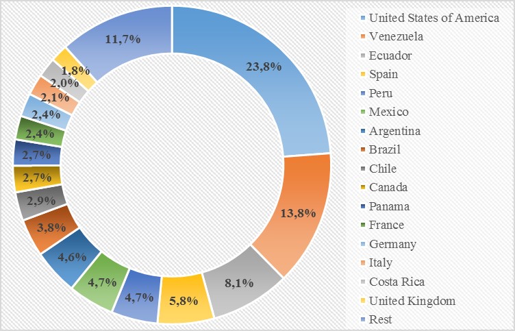
Source: own elaboration with UNWTO database (2016).
In addition, these trends in the relationship between the arrival of international tourists and physical distance to the main destinations in Colombia from different origins are synthesized more clearly in Figure 3 andMap 1. The largest bubbles represent the largest volume of visitors to Colombia, where 71.8% of visitors are from countries within an average of 2,739 kilometers of linear distance; this relationship is consistent with the gravity model indicating a greater tourist flows where the distances between the origin and the destination are smaller.
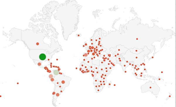
Source: own elaboration using data from UNWTO (2016) and the Google Drive mapping tool.
Table 1 summarizes the descriptive statistics of the balanced panel. As mentioned in the methodology, quantitative variables were transformed through natural logarithms. A considerable variation is to be observed for most variables, owing to the heterogeneity in the sample of countries studied.
Source: own elaboration. The quantitative variables are expressed in natural logarithms.
4.2. Linear Mixed Model
The response variable used in the first estimated LMM is the natural logarithm of tourist arrivals. In all, 166 countries were examined, each one of them with 18 instances of data, for a total of 2,988. Among the explicative variables used to estimate the model, GDP per capita, and the real exchange rate are determined for each year, as were the clusters found using R’s pam function. Missing data were allocated using statistics, as the median of the arrival’s variable.
Cluster variables were generated in the estimation of the models due to the heterogeneity of the response variable. The process is completed before the model is estimated and consists of grouping data according to their common characteristics; therefore, seven groups are generated by grouping similarities and clusters are used as a factor for improving the adjustment. For example, countries with the shortest distance to Colombia are located in cluster five.
The LMM under the Normal distribution has a low adjustment capacity because of the response variable nature, since it does not have a continuous form. In this sense, high scores are found for SMAPE = 113.9% and RMSE = 4654.7, indicating a considerably poor adjustment. Hence, a transformation is unnecessary; Gaussian approximation is inappropriate in this case. For this, it is necessary to create a model with a Poisson response.
4.3. Generalized Linear Mixed Model (GLMM), with a Poisson response
Given the counting response for the variable of tourist arrival, a Poisson response model was estimated. For this, the response variable is the number of tourist arrivals, which was given as an integer. The explicative variables were similar to those from the previous model. When estimating the GLMM, a single random effect was used, the intercept, obtaining the estimated coefficients seen inTable 2; these may be seen as significant at a 5% level. The distance variable (transformed by the logarithm), became non-significant; therefore, it was eliminated from the model and another model was re-estimated without it. In other models with more random effects, this variable has significance at a 5% level. Column 2 ofTable 2 shows the effect value, indicating that variables with a higher effect on increase are the natural logarithm of year, followed by direct fly (binary; it is 1 if there is a direct fly, otherwise 0), followed by language (binary; whether the countries share a language with 1 or not with 0). Column 5 shows the p values, demonstrating that all variables are significant because they are lower than the alpha significance level of 5%. It is not clear that distance has explanatory power, but this is found for variables such as visa, which indicates a decrease in the travelers if visa is required; and language, which increases the number of travelers if there is a common language.
Source: own elaboration using the lme4 package for R.
Further, this shows that visa requirements reduce the arrivals, since the mean of the behavior of arrivals for visa requirements, 156.63, is lower than the mean of the arrivals for countries without visa requirements, 11178.78. This result also confirms the correlation among arrivals and the logarithm of distance, which is negative, −0.27, and the correlation among language sharing, which is positive, 0.425, as well as the negative correlation among real exchange and arrivals, −0.0668. These results indicate that a substantial amount of tourism comes from countries that are close to Colombia; it would be interesting to know the specific activity of the tourist in order to conduct a more advanced diagnostic and subsequently propose strategies aimed at improving care.
The estimated generalized mixed model has a better adjustment; this is reflected in a decrease in the SMAPE indicator, 49.7%, and an RMSE of 2979.98. Similar to this GLMM, other models were estimated by adding more random effects. Summary adjustment statistics are shown inTable 3. The best-fit model has four effects.
| Number of Random effects | 1 | 2 | 3 | 4 |
| SMAPE(%) | 49.723 | 41.815 | 39.517 | 37.596 |
| RMSE | 2979.98 | 2688.07 | 2730.48 | 2541.21 |
Source: own elaboration using the lme4 package for R.
4.4. Bayesian Generalized Linear Mixed Model, with Poisson Response and a Random Effect
The response variable, arrivals, is the same as the one used in the previous models. The prior distribution of fixed parameters is the Normal one. The covariance matrix has a non-informative distribution for this model.Table 4 lists the fixed-effect values in Column 2 (Estimate) and the p values (referred to as Pr(>|z|) in Column 5), with values lower than 5% indicating the significance of all the variables that remain in the model. It is observed that distance is significant and shows a negative value, which indicates that the greater the distance, the fewer the tourists, consistent with the descriptive statistics. In addition, effects on time are positive, showing increase in tourism over the years. According toEilat and Einav (2003) andVargas et al. (2007), exchange rate indices have a negative effect; that is, the lower the value of the exchange rate, the higher the tourist flow. This model estimation is opposite because the higher the value of the exchange rate, the lower the value of tourists. In addition, the political index and GDP are positive, showing that countries with a greater political stability and a higher growth are those that visit Colombia most often; this has also been documented in other studies, such asNaudé and Saayman (2005) andEilat and Einav (2003). In this specific case, it should be noted that the there is a change in the perception of the country’s security conditions, such that the number of visitors shows an increasing trend over the years, despite this variable being perceived as a risk by tourists (Vanegas 2015).
Source: own elaboration using the lme4 package for R.
The Bayesian model has a better adjustment with respect to the normal model (113.9%), which is reflected in a decrease in the SMAPE error indicator to 49.7% and an RMSE of 2967.59. Furthermore, as more random effects are added to the model, the adjustment improves, as seen inTable 5. Thus, the adjustment indicators for the Bayesian models show models with one, two, three, and four random effects; this is similar to the previous GLMM model type, wherein the model adjustment quality is improved when the number of random effects is increased. In addition, in the first case (one random effect), a non-informative distribution was used for the fixed parameters; however, from the second onwards, the prior Normal distribution was used, and its benefit can be seen in the lowest SMAPE values (38.66%), with RMSE = 2005.83 and coefficient values consistent with those of the other models, therefore, that model is chosen as the best model.
Real exchange rates represent important effects in GLMM, but price is also important and economically different. The first measure considers the competitiveness of tourism services; relative prices measure a country’s economic lifestyle (in effect, explaining how expensive a country is). Statistical forecasting techniques and econometric models can consider two non-linear combinations (time and quadratic time) for one variable and take advantage of the statistical learning required to optimize the adjustment.
To test the consistency of the REER effect, with or without price, a sample including different countries (from Europe and North America), shows the same negative value in the model’s effect. This result is consistent with trends observed in countries such as Argentina and Costa Rica. In addition, 11 of 42 countries (26%) had negative correlation values among arrivals and REER, and 19 (45%) had a correlation below 0.3. Globally, 49 of 166 countries (30%) had negative correlations and 89 (54%) had a correlation below 0.3. This result uses a current estimation strategy called statistical learning, which achieves advantages from the data by decreasing error and variability. For example, using variables as clusters, as well as others related to dollar values and relative prices, improves the estimation and is consistent with other statistics, such as correlations.
However, it can be seen that the overall effect of lree and the correlation is negative and significant regarding tourist arrivals. This indicates that the negative effect of this covariate has a prevailing influence on tourist arrivals.
| Number of Random effects | 1 | 2 | 3 | 4 |
| SMAPE(%) | 49.70736 | 41.63011 | 39.85239 | 38.65872 |
| RMSE | 2967.586 | 2771.549 | 2731.578 | 2005.825 |
Source: own elaboration using the lme4 package for R.
Common effects are found in the different modeling approaches. Time has a positive effect on tourist flow; namely, there is a positive tendency in that the number of arrivals is higher as time progresses. In addition, in most models, where distance is significant, it is inversely proportional to arrivals (different from the information shown in the panel data model); that is, the greater the distance, the fewer the number of tourists. This is, however, not significant in many models. Conversely, the exchange rate always has a negative effect, such that the higher the value of the dollar, the lower the number of tourists. The fact of bordering Colombia also increases arrivals; the arrivals decrease with respect to the countries for which visas are required. In some cases, a common language appears to be significant with a positive value, indicating that sharing a language increases the amount of arrivals. Having a direct flight is also related positively to tourist flow.
5. CONCLUSIONS
A review of the literature shows that significant factors for tourist attraction to a destination include the development conditions in the country, incomes, relative prices, exchange rates, and travel costs. Other factors are distance between countries, geographical conditions, and institutional conditions. Some hypotheses found in the literature, such as the inverse relation of distance with the entry of international tourists, were tested in this study. GLMMs reflected some relevant variables in all estimated functional forms, such as how the variable for common border and language was linked with increasing tourism; this allowed for evidence to be provided for the associations raised.
The findings for the most important results of literature show that certain economic variables, such as exchange rate, GDP, and political stability indicators, are determinants for tourist flows to Colombia. The depreciation of the peso-dollar exchange rate provides a greater motivation for inbound tourism, a motivation that is also found in countries with better security guarantees and economic and political stability, verifying the information that found in other tourism studies. Conversely, the variable of distance has a significant effect in some GLMMs with an inverse effect on tourism because distance presented significant negative effects, indicating that people from the nearest countries travel more, which verifies the information shown in the descriptive graphics and is also in accordance with the literature reviewed. Countries sharing a language or having a high percentage of Spanish speakers with high political indices result in large numbers of visits to Colombia. The category of shared official language includes Spain, and the category of having a large number of Spanish speakers includes the United States. Thus, these countries send large numbers of visitors, although these countries are not close to Colombia. Although there has been a historical link with the countries of the Andean Community, there are fewer visitors. Tourism dynamics also reflect the existence of positive trends, as was observed in the high value and significance of the coefficient accompanying time.
The results obtained by this work may be useful for decision makers in the tourism sector. Policymakers may resort to the knowledge of the variables, those that may have an impact on the basis of their policies, to support and strengthen the growth of the tourism industry. This is of greater importance when the attention addresses the impacts entailed by the peace agreements signed by the guerrilla forces that exerted control over territories with high potential for tourism. In this sense, policies could be oriented to leverage territorial development. Projects oriented toward the sustainable management of these territories’ biocultural assets are exploited by the communities that propose undertakings around scientific tourism. In addition, a community’s appropriate scientific knowledge relates to its existing environment, ecosystem, and biocultural relationships. Contributing to these regions’ development are income-generating, sustainable, community-based tourism alternatives. These programs eschew large volumes of tourists in favor of more specialized tourists who have the potential to produce the same or greater amount of income.
In summary, initiatives that avoid high-volume tourism’s social and environmental problems with a more responsible solution will change a country’s form of tourism. This should produce positive impacts while simultaneously preserving the systemic and socioeconomic conditions of tourist areas, which were controlled by illegal forces in the past. Finally, some of the results show a growing number of necessities for optimizing strategies such as adequate planning, improving services, and enhancing tourist attraction, for example, through marketing strategies, resource management, or increasing inventory stocks in hotels for the more affluent tourism periods.