
INTRODUCTION
Due to the increasing demand for energy, the extraction of renewable energy sources comes into focus increasingly frequently. Renewable energy has different sources depending on the potentials of the location.
By reviewing the global market of renewable energy sources, we can see a growing trend from year to year. By the study of Frankfurt School – UNEP Collaborating Centre for Climate & Sustainable Energy Finance[1] in 2018, the estimated new investment was 133,5 billion USD for solar, 129,7 billion USD for wind, 6,8 billion USD for waste energy technologies, such as biomass, 2 billion USD for geothermal, 481 million USD for biofuels, and 359 million USD for small hydro powers. The overall estimated new capacity installation cost was 272,9 billion USD, which is less by 12 % compared to the new investments in 2017. Researchers have been working on improving the power cycle efficiency in order to decrease the cost of renewable energy. For example, the use of supercritical CO2 as working fluid in power cycles has the potential to revolutionise power generation2.
In the urban area where usually a traditional energy system is available, several base power plant provides the electricity. In contrast to the traditional system, in the smart grid next to the base power plant there are variable energy sources, i.e. renewable energy sources. The strength of this system is that any small scale energy sources could be the main power plant for a sub-system for a required time interval. For example, for small electrical devices like a coffee machine PV panels or small scale wind turbines could complete the available big scale power plant’s electric production.
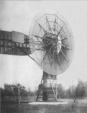
Focusing solely on the wind energy sector, the first wind turbine (WT) was invented by James Blyth in 1887, which was a vertical axis wind turbine (VAWT). The first horizontal axis wind turbine (HAWT) was invented by Charles Brush and built in 1888. This two WTs are shown in Figure 1.
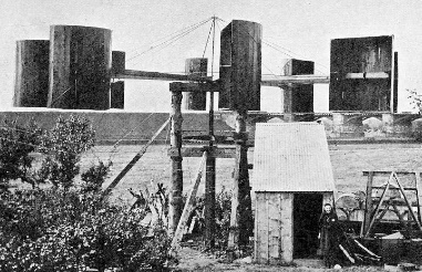
While the first WT’s structures were constructed of wood and canvas, nowadays turbines are constructed of steel, concrete, glass fiber and epoxy matrix composite materials. Thanks to these new materials and the growing demand for electricity, an increasing number of WTs appearing in the cityscape.


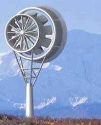
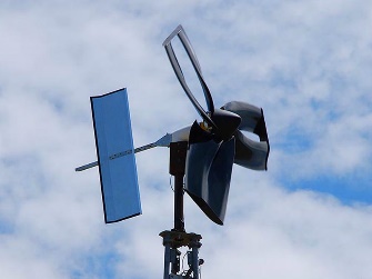
Nowadays, due to the development and installation of a growing number of WTs, it is important to examine how multiple wind turbines in close proximity interact with each other and with the installation areas, such as buildings in the urban region. A. Nagy and I. Jahn[7]398 have shown a measurement system that is capable to measure flow parameters between wind turbines. The technology of WTs is evolving continuously to be more autonomous, sustainable and economical. Innovations helped in the development of new parts, e.g. guide baffles, new blade structures and profiles, some of which are shown in Figure 3.
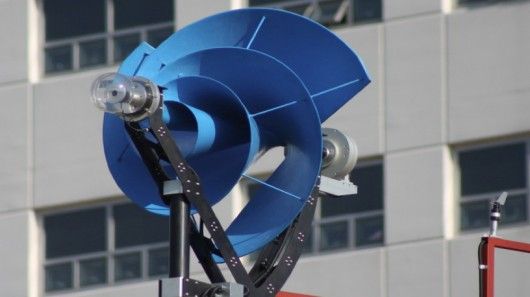
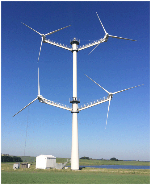
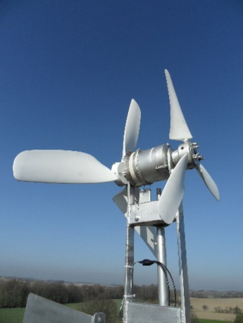
The layouts of multiple “standard” turbines used on the same tower may only be limited by imagination, as new structural innovations are being considered. There are different approaches when the turbines are installed on different axes or on the same rotating axis. For the latter type, depending on the rotating direction, the turbines are called co-rotating or counter-rotating dual rotor wind turbines (CR-DRWT and CO-DRWT). These unconventional WTs are shown in Figure 4.

Lee et al.[14] simulated a CO-DRWT’s power coefficient, cp by using the blade element momentum theory and they compared it with a cp of a traditional single-rotor wind turbine (SRWT). As a result, the CO-DRWT showed in some cases higher performance for different pitch angle, rotating speed and radius ratio compared to the SRWT.
The power coefficient, cp, which we were refed can be calculated with the following equation:
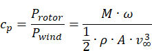
In the equation, Protor is rotor’s power, Pwind is the wind power, M is the torque, ω is the angular velocity, ρ is the density of the air, A is the swept area, v∞ is the freestream velocity.
Ozbay et al.[15] performed an experimental study to compare the power production performance of CR and CO DRWTs compared to SRWTs. They found the DRWTs’ overall cp was higher than the SRWT’s. Furthermore, they found that the counter-rotating DRWT can harvest more energy than the co-rotating DRWT.
Theoretically, cp has a maximum value, which was calculated as 16/27 (59,26 %) by the one-dimensional Betz’s law, and 30,113 % by the two-dimensional GGS model[16]. By the measurement results for the SRWT, the maximum efficiency was shown to be in between the GGS and the Betz limit.
MOTIVATION
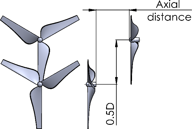
In this research, a CO-DRWT was studied without the tower and a nacelle. In our analyses, the propeller layout was chosen as being fixed as 0,5D radially, and with a variable axial distance between 0,005 and 2D. (The D in the distance values represent the rotor diameter, which was 200 mm.
For the initial position, the 180° shifting between the mirrored wheels “top” planes were selected to avoid overlapping between the blades. The initial geometry and the labelled distances are shown in Figure 5.
By numerical simulation, cp values were calculated and compared for the studied cases.
SIMULATION AND EXPERIMENTAL METHODS AND SETTINGS
In the next subchapters, the finite volume method (FVM) is reviewed for the simulations, and our simulation’s boundary conditions and measurement system are described.
SIMULATION METHOD
In the simulations, two different CFD (Computational Fluid Dynamics) software were used with the finite volume method.
The FVM divides the computational domain into finite volumes, and using the conservation laws (mass, momentum and energy) to compute the flow field properties. This calculation uses the transport equation of:
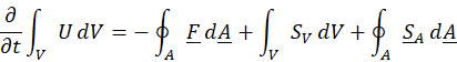
In the equation, 𝜕𝑈𝜕𝑡 is the time-dependent member, U is a residual quantity’s volumetric flux, F is the same residual’s flux, SV is the F flux’s volumetric source, SA is the F flux’s surface source, V is the computational volume and A is the computational volume’s surface.
The CFD codes solve this equation and its linked equations iteratively until the residual quantities do not decrease to a prescribed (near zero) value.
SIMULATION PARAMETERS
For the simulations, Mentor Graphics’ FloEFD and Ansys CFX were employed.
In each simulation, we used air from the software’s material database, which enters to the domain at the inlet face with 3,79 m∙s-1 freestream velocity. The outlet faces had an environmental pressure of 1 atm, where the flow could quit from the domain. The wind turbine tip speed ratio was 4, which means the rotating region had 24,1279 RPS angular velocity.
For clarity, the tip speed ratio can be calculated by equation (3), where 𝜆 is the tip speed ratio, ω is the angular velocity, R is the blade’s radius and v∞ is the freestream velocity.

The simulation with FloEFD was in steady state with frozen rotor technique, and transient with the sliding mesh method. The unsteady simulation was run for 0,4144582 second, which is the time requirement for 10 rotations. In each state the k-ε turbulence model was used.
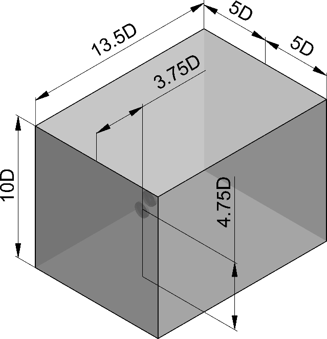
In FloEFD, its own mesher was used, which provided a cartesian mesh with cell mating and cut-cell methods. For these simulations a rectangular computational domain was used (Figure 6).
For CFX, nearly the same boundary conditions were used as in FloEFD, with the following differences:
for modelling the turbulence, the SST model was used,
for meshing the body fitting and element sizing technique was used,
a tubular computational domain was used (Figure 7).
Two different methods were used, the frozen rotor method (in steady state) for sweeping the whole axial range, and the sliding mesh technique (in unsteady state) for simulating the turbulence and checking the steady state result for the measured axial distance.
MEASUREMENT METHOD
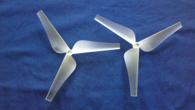
For validating our simulation, a 3D printed version of the turbine wheels were used, which are shown in Figure 8.
The printed wheels were taken into a wind tunnel (Figure 9) where we were able to measure the generated torque[17].
RESULTS
RESULTS
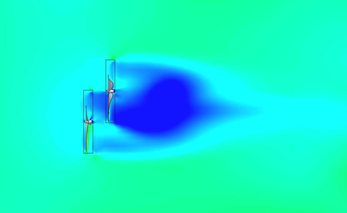
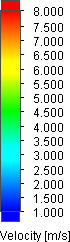
In the software for each axial distance the flow field was similar. In the next figure (Figure 10) the velocity distribution near the turbines for A = 0,5D distance is shown.
For comparing our simulations, we were monitoring the torque on the surface of the blades. At the end of the simulation, in steady state the simulation affords a single value for the torque, while in transient the CFD software a torque value was produced for each time step. These time series are shown in Figure .
The power coefficient (cp) can be calculated from the torque and the boundary conditions. In Figure 12 the simulated cp-s is shown, the frozen rotor technique (steady state) with blue dots, and the cp with SST turbulent model in unsteady state (CFX) with the yellow square, and the cp with k-ε turbulent model in unsteady state (FloEFD) with grey diamond, and the measured cp with the red triangle. In each case, the cp value is the sum of the two blades’ power coefficients.
The simulated cp with frozen rotor was 96,54 % while the simulated cp with transient rotor stator was 86,15 % (with SST) and 86,08 % (with k-ε) of the measured cp.
For comparison, we ran a simulation with frozen rotor technique for a one rotor turbine, and its power coefficient was 0,3424, which was 73,29 % of the measured CO-DRWT’s cp.
CONCLUSIONS
In this study, we were analysing a counter-rotating dual rotor wind turbine between 0,005D and 2D axial distance with a fixed 0,5D radial shift. At the end of the simulations, the power coefficient was plotted against the axial distance (Figure 11), and it was compared with a measured value.
Upon the results shown in Figure , the following statements can be established:
1) The power coefficient (cp) was higher when the turbine wheels were closer.
2) In a built application, the zone before 0,2-0,25D was avoided, because the blade deformation could cause collisions.
3) The highest cp was found at 0,05D. The second was at 0,005D, which is 0,01096 % smaller than value at A = 0,005D.
4) The dependence of the simulated cp’s with the distance can be modelled as y = –0,0172 ∙ x4 + 0,0487 ∙ x3 + 0,0370 ∙
x2 – 0,1792 ∙ x + 0,5343 with the goodness of fit of R2 = 09874.
5) The first wheel power coefficient (cp1) and the second power coefficient (cp2) were approximately the same in the 0,05-0,25D range.
6) After 1D axial distance, the cp1 value was 3 to 4 times larger than cp2.
7) The SRWT’s cp value was 4,29 % larger than CO-DRWT’s cp1 value for the 1.5D distance, 4,25 % more than the 1,75D’s value and 3,01 % bigger than the 2D’s value.
Upon conclusions 1) and 2), the recommended optimal distance was the closest where the blades do not have any collisions. For the required minimal distance, a measurement or a two-way FSI simulation is necessary.
We made the mesh dependency analysis for the A = 0,5D configuration, therefore, conclusion 3) might be a result of a numerical error. If not, the cp of 0,05D has the largest value, therefore, it is energetically the best examined distance.
Regarding conclusion 7), we can establish that for large axial distance (like the 1,5-2D), a counter-rotating DRWT first rotor produces similar power like a single SRWT, therefore, the second rotor produces the extra power.
Based on the conclusions of the presented study, the CO-DRWT has a large potential as an engineering application for increased wind energy harvesting at small places where it is needed, such as in the urban areas of smart cities.