1. INTRODUCTION
The total energy consumed in heating, ventilation and air-conditioning (HVAC) systems in commercial and residential buildings nowadays accounts for 40% of global energy consumption (37% in Argentina) and causes more than 36% of CO2 eq. emissions[1]. Optimizing energy consumption while maintaining thermal comfort conditions for users has then become a priority. This paper deals with the development of a dynamic model that describes the variations in thermal and humidity factors within a workspace located in the Faculty of Engineering at the National University of San Juan (UNSJ), an arid zone of Argentina, during the summer season. The climate in this city is continental, with high temperatures and low humidity in summer, as described in the national standard IRAM 11603[2]. The main variables to be modelled are the user´s thermal comfort and the energy consumption of the HVAC system.
The final goal is to implement a Multi-objective Predictive Optimizing Control of the air conditioning system[3]. This type of supervisory control performs multi-objective optimisation[4] since it considers factors that normally compete with each other, such as user comfort and energy consumption. It performs this optimization with a Model Predictive Control (MPC) strategy[5], that is, running the model forward in time in order to calculate the optimal control actions. A well-suited model is the main challenge when implementing predictive control, especially when applying it to comfort and energy efficiency[6].
Different models describing how buildings react to external variables and climate control are discussed in reviews such as those by Afram and Janabi-Sharifi[7] and Homod[8].
The models are frequently classified as white, grey, and black box models based on their level of transparency. Arendt et al.[9] have carried out an appropriate comparative analysis of these modelling criteria for the simulation of the thermal behaviour of educational buildings. Similar classifications using different terminology have also been established. Hensen[10], for example, defines four levels of models, from a Conceptual one, in which an ideal plant is considered, to an Explicit one, which has precise knowledge of the different subcomponents of the system in terms of energy balance. The traditional black and white box models can be identified with these extremes.
In a white box model, the internal details and underlying mechanisms of the system being modelled are known and taken into account. It requires a comprehensive knowledge of the physics involved, the components used and the boundary conditions of the modelled object. Normally, the changes over time are determined by solving the differential equations that explain the process using numerical methods.
White box models have been widely used in environment modelling. For example, Muñoz et al.[11] used the admittance method to thermally characterize multilayer wall materials. Tashtoush et al.[12] present a dynamic model of an air-conditioned space that includes the physical details of the space, heating, cooling and dehumidifying coils, humidifier, ductwork, fan and mixing box. Commercial software packages like ESP-r and TRNSYS[13] are commonly used to predict the thermal performance of buildings. These programs have been developed with a deep understanding of the physics and materials used. Assessing alternatives for retrofitting environments and HVAC systems is another valuable application for these programs[14]. On the other hand, white box models have the disadvantage that they require a precise knowledge of the physical parameters of the different elements involved. The incorrect parameters can lead to significant differences between the actual behaviour of the system and the behaviour described by the model. This has been emphasized by authors like Akkurt et al[15]. Some researchers also argue that the calibration of these models in the case of complex buildings is cumbersome so the application of predictive control is only possible for simple environments[16]. For these reasons, some authors such as Trcka and Hendsen[17] place this type of model in the category of models used for Building Energy Performance Simulation (BEPS), rather than in the category of models used for control and optimization.
At the other end of the spectrum, there is the black box model, which is named for its complete opacity. It is assumed that there is no knowledge of its internal structure, but it is based solely on observations of input and output data (data-driven). The techniques used to construct these models usually stem from the field of artificial intelligence and are often based on genetic algorithms[18] and, in particular, neural networks[19].
One of the main advantages of black box models is that they do not require detailed knowledge of the system. These tools are also useful when dealing with variables that have complex interconnections. However, its drawbacks arise from a high dependence on the quality of the input data. When the data used to calibrate the model are not reliable or do not cover all possible situations, the results obtained may deviate significantly from reality. For the same reason, they are difficult to correct or modify.
Grey box models lie between the two types of models mentioned above. Some structural features of the model are assumed, such as the orders of the transfer functions and the internal influences between the different variables involved, and the parameters of these models are determined by analysing the input and output data.
The approach to a grey box model can follow two basic ideas:
Models can be based on physics equations, but instead of deriving their parameters from knowledge of the individual components, they are calibrated on the basis of recorded measurements.
Generic models with a certain structure, e.g., in state space or using linear or non-linear input/output transfer functions, can be adopted, and records of measurements over time can also be used to estimate model parameters.
In the latter alternative, different approaches can be considered. Among the most common are:
Linear state space models. These models are useful when the environment is modelled under relatively limited variations in the variables affecting the system (e.g., outdoor temperature), which allows the assumption of a linear relationship between inputs and outputs. State models represent the system intuitively when each state variable is identified with some determinant value of the system's behaviour. With this idea, Drgona[20] uses a fourth-order state model, where the state variables are the external facade temperature, the internal facade temperature, the floor temperature and the internal room temperature.
Fuzzy logic. Prior knowledge about the system is expressed in terms of labels and linguistic rules and the parameters of these rules are then identified[21].
Linear transfer functions, either in the continuous or discrete domain.
Non-linear descriptions. When the behaviour of variables is complex and cannot be properly described by linear models, it can be verified that non-linear relationships exist between them. A non-linear description can also take different forms, such as states or non-linear differential equations. In this work, a Linear Parameter Varying description (LPV) is used[22] because it is very effective and easy to understand for those who know the behaviour of the system, which facilitates the identification of the parameters.
Once the model structure is defined, the usual techniques for determining the model parameters include, among others, the frequency domain method, the maximum likelihood method, and, above all, the Prediction Errors Minimisation PEM method, which is performed using least squares. This criterion must be supplemented by other model quality metrics in non-linear cases. This applies to certain sub-models described under the LPV criterion, which are discussed in more detail below.
Grey box models tend to have slightly larger prediction errors than black and white box models. However, they are very suitable for implementing an MPC because at each sampling interval, the controlled variable is measured again and the model is re-run from that point, so it is not the exact value of the prediction that is important but its trend.
It is generally agreed that a simple grey box model is sufficient for implementing an MPC[6]. They are also more robust (less sensitive to parameter errors) and perform better when the operating conditions differ from those under which the parameters were calibrated.
Given these considerations, the following model was chosen for this work:
Grey box dynamics.
Of an ambient and its HVAC system in the post-occupancy phase.
Aimed at multi-objective optimisation of user´s comfort and energy efficiency, in summer.
Characterized by low-order transfer functions, albeit with significant pure delays.
Most transfer functions are linear and, in some cases, LPV descriptions are used.
2. THE ENVIRONMENT, ITS HVAC AND RELATED VARIABLES
The set under investigation is shown schematically in Figure 1. The dimensions of the workspace are 7.2m long, 4.9m wide and 3.25m high and it is used for research and development tasks. The average occupancy rate is between 2 and 3 people for 6 hours on working days. As a boundary condition, it has a single wall -1- that is in contact with the outside world and lets in air and natural light through a window. As it faces south, it never receives direct sunlight. The other walls are connected to other workspaces and an indoor corridor, the ceiling to a room upstairs and the floor to the natural ground. All these conditions explain the good insulation and consequently the high time constants, in the order of hours, for the influence of the outside temperature on the internal variables. While the characteristics of the space primarily favour thermal comfort, the harsh summer conditions in this area require air conditioning, which consumes significant amounts of energy. It should also be noted that the system presents a challenge for automatic control as it has high pure delays with respect to the time constants involved.
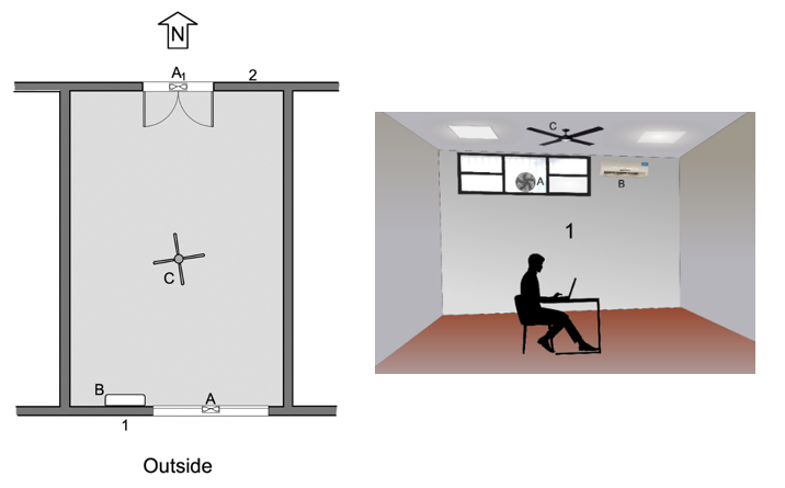
Fig. 1 Ground plan and view to the south of the room under study and its air-conditioning devices
The entrance to the workspace is located on Wall 2, opposite to Wall 1. A blower 'Fan A' located in the window on Wall 1, in conjunction with an exhaust fan over the entrance door on Wall 2, 'Fan A1', forms a variable-speed forced ventilation system (with speed denoted as va), which draws in outside air and circulates it through the room along its longest axis. If outside air is not supplied, an additional ceiling fan, 'Fan C', also operating at variable speed va, can generate an indoor airflow. This ventilation system serves a dual purpose: it equalizes the temperatures in the room and improves the occupants' sense of comfort by promoting convective heat transfer from the body to the surrounding environment.
The HVAC unit B operates at 220V, 50Hz and has a split configuration and ON/OFF operation, like most HVACs in Argentina. It blows the air at 1000 m3/h. The cooling power consumption is 1915W and has a cooling capacity of 6150W[23]; with these data, the Seasonal Energy Efficiency Ratio SEER[24,25] is 6150W / 1915W = 3.2, indicating that it is a mid-efficiency device. This underlines the idea of the need for optimisation, the ultimate goal of the project in which this study is embedded.
Three temperatures, the ambient humidity and the power consumption of the HVAC systems are measured and then modelled. The measured temperatures are the outdoor temperature Te [°C], using a sensor located outside the Wall 1, the ambient temperature Ta [°C], measured at 1.1m above the floor[26] in the middle of the room (under the ‘Fan C’), the mean radiant temperature Trm [°C][27], measured at the same location with a balloon temperature sensor, and the temperature associated with the HVAC unit Taa [°C], measured with a sensor at the top air inlet of the HVAC unit, also near Wall 1, see Figure 2. The linear distance between the measurement points of Taa and Ta is approximately 4m.
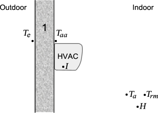
Fig. 2 Relative position of the measurement points, not to scale
The Taa temperature measurement has a dual purpose: On the one hand, when the HVAC is in operation mode, it is equivalent to the temperature measured by the HVAC's inside sensor and is then used to predict when the compressor unit device will be in the ON or OFF state. On the other hand, this point indicates the internal temperature of Wall A when the HVAC is not operating. Other sensors could have been placed on each of the other walls, but as they behave adiabatically, this was sufficient to get a proper model.
Humidity H [%] is measured relatively, as the amount of water vapour in the air, expressed as a percentage of the maximum amount the air can hold. It is measured at the same point as Taa and Trm. The measurement of the current consumed I [A] by the HVAC is used for energy calculations.
3. MODEL DEVELOPMENT
The inputs of the entire model are the reference temperature (or setpoint) SP [°C] at which the HVAC operates, the air speed va [m/s] and the outdoor temperature Te [°C] as a perturbation. See Figure 3.
The primary variables to be modelled, mentioned above in Section 2, allow the calculation of the variables relevant for the optimisation: the thermal comfort, expressed as the percentage of dissatisfied users Disc, and the energy consumption, expressed as a relative power Pr. Both will be formally defined later.
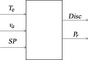
Fig. 3 Block diagram of the whole room-HVAC system
To obtain the sub-models presented below, various datasets obtained from different experiences of measuring signals over time were used. These covered the typical outdoor temperature ranges of the city in the summer season, between 15°C and 45°C, and different time evolutions of the outdoor temperature Te, with increasing and decreasing daily averages. As is usual for dynamic models, identification was made with the dataset of one experience, using the data of another experience to validate the obtained model. The final model, achieved by iteration of this methodology, properly reproduces the behaviour of the variables for all the experiences included in the identification.
3.1 Influence of the outside temperature through the envelope
The energy transfer through the envelope, without the operation of the HVAC, primarily affects the temperature associated with the inside of the wall Taa and, thus, the other variables. The more detailed version of the block diagram of the model is outlined in Figure 4.
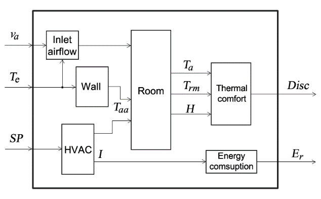
Fig. 4 Block diagram with internal influences
The change in wall temperature due to outside temperature, denoted as Taae, was adequately described by a linear transfer function in the discrete domain with parameters obtained by PEM. With a sampling interval of 0.0667 min, it has the following form:
In the identification process, an attempt was made to choose the lowest order of the model that maintains a bounded error, as in the following cases. Figure 5 shows the comparison between the measured variable and its model in an experiment of just over 3 days with typical variations in total outdoor temperature Te between 10°C and 25°C.
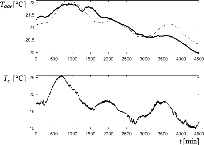
Fig. 5 Influence of the outside temperature on the wall temperature; The filled line is the actual output and the dashed line is the model output
The discrete transfer function Gaae acts on the differences between the two values Taa and Te with their mean values, denoted as and . The average value of Te is extracted using a high pass filter HPF, see Figure 6. To obtain the absolute value of the output, a constant value must then be added.

Fig. 6 Block diagram of the model of the dependence of wall temperature on outdoor temperature through the envelope
The combined effect of the pure delay and the time constants involved results in a total delay between input and output temperature peaks of about 4.5 hours for a daily sinusoidal input. See Figure 7.
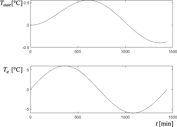
Fig. 7 Response of the wall temperature model Taae to a daily sine wave variation in Te
Similarly, the influence of the outside temperature on the ambient relative humidity He can also be determined.
The block diagram has the same structure as the temperature diagram in Figure 6. The comparison between the actual output and the model is depicted in Figure 8.
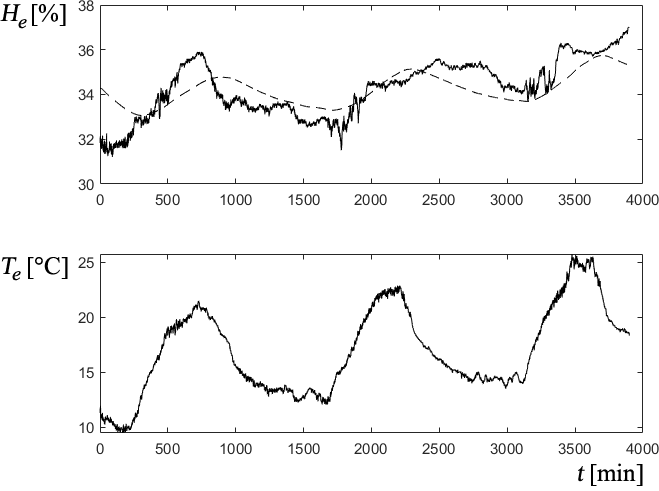
Fig. 8 Response of the Humidity model (dashed line) in relation to the outdoor temperature
3.2 Influence of outside temperature through forced cross ventilation
This ventilation occurs when the outside air enters through Fan A in Figure 1 and exits through its counterpart exhaust fan located on the opposite wall. Modelling this influence is important because as long as the outdoor temperature is lower than the indoor temperature (mainly at night), significant temperature reductions can be achieved to reduce energy consumption during the day.
The following identifications of the influence of the outside air flow on temperatures and humidity are presented in the same experience, in order to be able to make an appropriate comparison.
3.2.1 Influence on wall temperature Taa
The following observations can be made when testing with different air velocities (Figure 9).
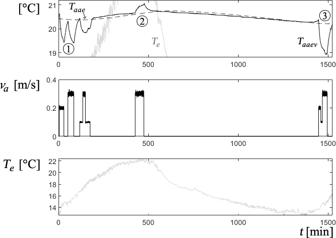
Fig. 9 Influence of the outside temperature (grey line) on the wall temperature due to forced ventilation
Looking at the behaviour of the wall temperature due to the combination of the external temperature and the air velocity Taaev, compared to that which depends only on the external temperature Taae through the envelope (identified in the previous point and plotted here in dashed line), it follows that it increases when Te > Taae (state 2 in the graph) and decreases the other way round (states 1 and 3). This makes sense. When warmer outside air is brought into the room through the ventilation, the internal temperature tends to rise, and vice versa. This suggests that the influence of the outside temperature by the air supplied from outside Gaaev should be modelled as a function of the T’Δeaa difference between Te and Taae and then added to the latter. See Figure 10. This considers the effect of external ventilation.

Fig. 10 Block diagram showing the influence of the outside temperature on the wall temperature, both through the envelope and the forced cross-ventilation
2. The experiment in Figure 9 also shows a predictable effect of air speed va in which the outside temperature affects the other variables. Not only does the effect of Te on Taa increase with air speed, suggesting a dependence of the static Gaaev gain on this variable. In addition, the time constants involved also vary with different va rates. Taking this into account, Gaaev was modelled as a first-order system with pure linear delay with linear variant parameters LPV, where the three parameters of the model, Kav, tgav and tuav, are dependent on va.
In this case, the model is expressed in continuous time. This makes it easier to determine the parameters as a function of va.
Among all possible representations of the model parameters (3) as a function of the scheduling variable va (fuzzy, point interpolation, neural networks, etc.), a second-order polynomial form was chosen due to its simplicity.
Since this is a non-linear system, the PEM error minimisation criterion[28] must be supplemented by tests of independence and whiteness validity and other indicators of model quality to identify the parameters of these parabolas[29,30]. These are combined using a multi-objective strategy[31,32]. Using this technique, the variation of the first-order model parameters with va was determined as shown in Figure 11.
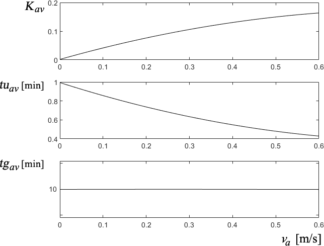
Fig. 11 First-order LPV parameters of the outdoor temperature under the influence of forced cross-ventilation
It can be observed that, as expected, there is no external thermal contribution at null air speed va, and the pure delay in sensing a change also decreases with speed. The fact that the time constant of the system is almost invariant is not so easy to predict. With these parameters, the model shown in Figure 10 behaves as shown in Figure 12.
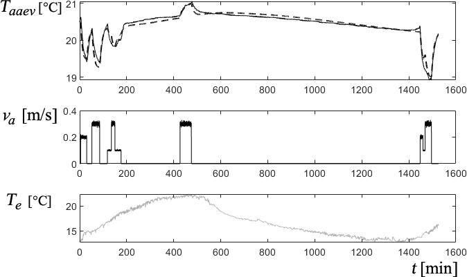
Fig. 12 Model behaviour of the outdoor temperature under the influence of cross ventilation (dashed line)
The influence of the outside temperature through cross-ventilation va on the ambient temperature Ta and the mean radiant temperature Trm is obtained similarly.
3.2.2 Influence on the ambient relative humidity H
When analysing the behaviour of the humidity with the external airflow, it can be seen that it also depends on the difference T’Δeaa between Te and Taae, but in the opposite direction: if this signal is positive, the humidity level will decrease and vice versa. This leads to the conclusion that it can also be described by a first-order LPV system Ghev similar to the one previously described, having a transfer function with the same structure as (2). The corresponding block diagram is drawn in Figure 13, and the temporal behaviour of the model in Figure 14. The evolution of the Ghev parameters with air velocity exhibits similar parabolas to those of the temperature shown previously in Figure 11 but with negative gains.
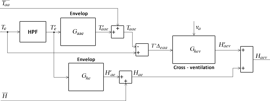
Fig. 13 Block diagram illustrating the influence of the outdoor temperature on humidity, both through the envelope and through forced cross-ventilation
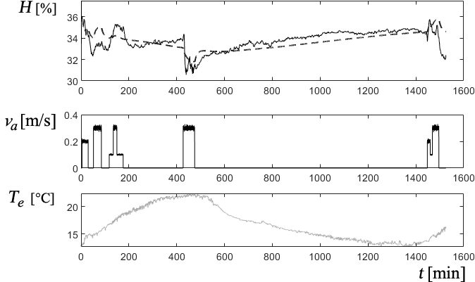
Fig. 14 Behaviour of the humidity model (dashed line) with the outdoor temperature, through forced cross-ventilation
3.3 Operation of the air-conditioning system
Looking at a typical test of the variables against reference changes in the HVAC, as shown in Figure 15, the following observations can be made.
The speeds at which the different variables move seem to depend on the operating range defined by the reference or setpoint SP set in the HVAC.
The ON/OFF behaviour of the HVAC causes the associated temperature Taa to move around the SP and the others (Ta, Trm) depending on the former.
The hysteresis ht with which the HVAC operates also depends on the reference SP.
The humidity also varies with the operation of HVAC. When the HVAC is in ON mode, it removes humidity from the environment by condensing it on the expansion coil, thus reducing the relative humidity H of the environment.
When the HVAC is in ON mode and the compressor draws power, the current consumption I is almost constant. Thus, a binary signal ua can be defined as 1 when the HVAC is ON and 0 otherwise, and a relative power Pr as:
where tp is a specific evaluation time of at least one ON/OFF switching cycle of the HVAC. As a result, Pr ranges between 0 and 1 and is equal to one if the HVAC compressor is always ON (ua = 1 always). This method of measuring the consumed power makes it possible to be independent of the absolute value of the consumed power [W].
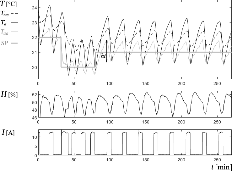
Fig. 15 Typical behaviour of variables under HVAC action
3.3.1 Influence on temperature associated with the HVAC and the wall Taa
This temperature tends to follow the wall temperature due to the outside temperature Taaev, already modelled in 3.2.1, when the HVAC is inactive (OFF mode, ua = 0). On the other hand, if ua = 1 permanently, the wall temperature tends towards the minimum Taamin that the HVAC can reach without switching off the compressor. This value can be obtained by means of a test by setting the SP reference to the lowest value it accepts. It depends on the average outdoor temperature. However, it can be considered constant for the summer period under consideration. This is illustrated in the block diagram in Figure 16.
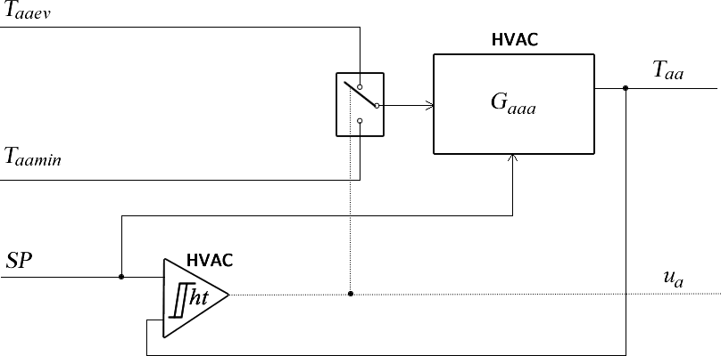
Fig. 16 Block diagram of the behaviour of the wall temperature associated with the HVAC
Similar to 3.2, the transfer function Gaaa is a first-order LPV system with pure delay similar to (3) but here the parameters vary with the SP of the HVAC. A multi-objective identification procedure similar to the one described above was also used to obtain this variation. It is depicted in Figure 17.
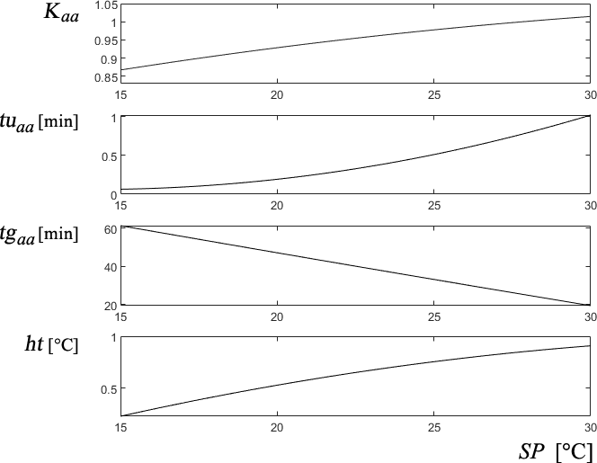
Fig. 17 Variation of the first-order parameters of Gaaa with the SP reference of the HVAC
3.3.2 Influence on the room temperature Ta and mead radiant temperature Trm
Following the same considerations as in the previous case, the experiments show that when the HVAC is inactive (OFF mode, ua = 0), the ambient temperature tends asymptotically to the wall temperature, which depends only on the outdoor temperature Taaev (see 3.2.1). In the opposite case, when ua = 1, it is determined by the total wall temperature Taa obtained in section 3.3.1 above. This can be represented graphically, as shown in Figure 18.
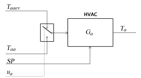
Fig. 18 Block diagram showing how the ambient temperature Ta depends on the operation of the HVAC
Again, the corresponding transfer function Ga is a first-order LPV model with pure delay. Its parameters change as a function of the SP reference, similarly to those shown for Taa in Figure 17. The behaviour of the mean radiant temperature Trm is similar, although with its parameters.
3.3.3 Influence on the relative ambient humidity H
The variations produced by the operation of the HVAC must be added to the Haev humidity produced by the outdoor temperature Te and the air velocity va previously modelled in 3.2.2. This influence was described using a linear system so that:
The complete comparison between the measured signals and their models is depicted in Figure 19.
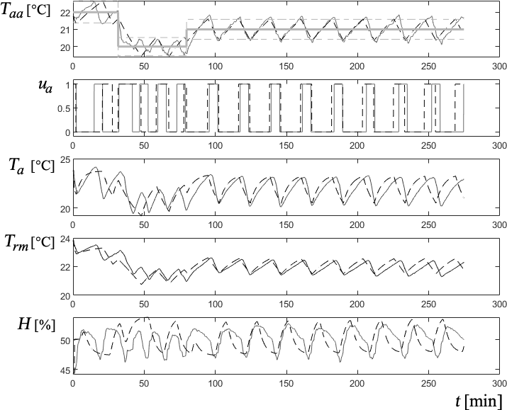
Fig. 19 Comparison between measured signals and their models, in dashed lines
3.4. Thermal comfort model
From the modelling of the physical variables described above, a measure of thermal comfort can be derived. The ISO 7730:2005 standard[33] defines it as "that mental condition which expresses satisfaction with the thermal environment" and postulates that up to 10% dissatisfaction with the thermal environment is acceptable. The standard does not provide a way to determine its measure. For this purpose, this study uses the equation proposed by Kuchen et al.[34], which estimates the percentage of dissatisfied users in the environment as follows:
This equation determines users' ability to thermally adapt to the evolution of the indoor climate by incorporating the operative temperature Top and the neutrality temperature Tn, defined below. This model was created based on the correlation of objective and subjective data obtained from 1300 measurements (Spot-Monitoring) in 30 office buildings in central Europe[34,35]. In this model, the minimum possible percentage of dissatisfied users is 7%.
According to the ASHRAE 55 standard[36], the operative temperature Top is an integrated temperature that fully influences the occupant's thermal perception of the thermal environment. The operative temperature is composed of the ambient temperature Ta and the mean radiant temperature Trm, according to the following equation:
where A is a factor that depends on the va air velocity in the environment, as shown in Table 1:
Table 1 Relationship between the air velocity va and the A factor
The neutrality temperature Tn is the value at which the individual perceives both physically and psychologically a pleasant environment that is neither cold nor hot. This condition corresponds to a comfort vote CV = 0 (neutral) on the 7 points of the ASHRAE 55 scale, as shown in Table 2.
Table 2 ASHRAE 55 scale
| Thermal sensation | cold | cool | slightly cool | comfortable or neutral | slightly warm | warm | hot |
|---|---|---|---|---|---|---|---|
| CV | -3 | -2 | -1 | 0 | 1 | 2 | 3 |
There is a linear relationship between the comfort vote and the operative temperature:
Where the parameters a and b can be established determined statistically through user surveys. The Tn neutrality temperature, the Top operative temperature and the CV comfort vote are related by the linear expression:
This expression shows that when the operative temperature is neutral, the user should emit a null CV. Constant c was obtained from the survey of the users' comfort votes. For the environment under study, described in section 3.2, these values are a = 0.3555, b = -8.8424 and c = 1/b = - 0,8869.
From the last equation, it is clear that:
This last value is finally inserted into Eq. (6) to determine the Disc percentage of dissatisfied users.
3.4.1 Effect of humidity on comfort
It is well known that when humidity is high, the air cannot absorb the evaporation on the skin, making it difficult for the body to release heat. This increases the user's sensation of warmth. Another factor that plays a role in this sensation is the speed of air. This has already been taken into account in Eq. (7). To consider the influence of humidity, the concept of thermal sensation or heat index Tts[37] is used. It was first proposed by Steadman[38] in his comfort model and expressed by Rothfusz[39] using the following polynomial form:
|
Tts = -8.784695 + 1.61139411 Ta + 2.33854883889 H - 0.14611605 H Ta - 0.012308094 - 0.0164248277778 H2 + 0.002211732 H + 0.00072546 Ta H2 - 0.000003582 H2 [°C] | (11) |
Alternative expressions for the heat index are given in the literature. Stull[40] even cites a third-order polynomial index.
The US National Weather Service[41] warns that this expression is not valid for combinations of high temperatures and humidities and that in certain areas it should be corrected using the following criteria:
If H < 13% and 26.67°C < Ta < 43°C the following adjusting value must be subtracted from (11):
If H > 85% and 26.67°C < Ta < 30.55°C the following adjustment value must be added to (11):
Finally, this simpler expression should be used when the ambient temperature is below 25°C:
Based on these criteria, the graph of the heat index as a function of ambient temperature and humidity is shaped as shown in Figure 20.
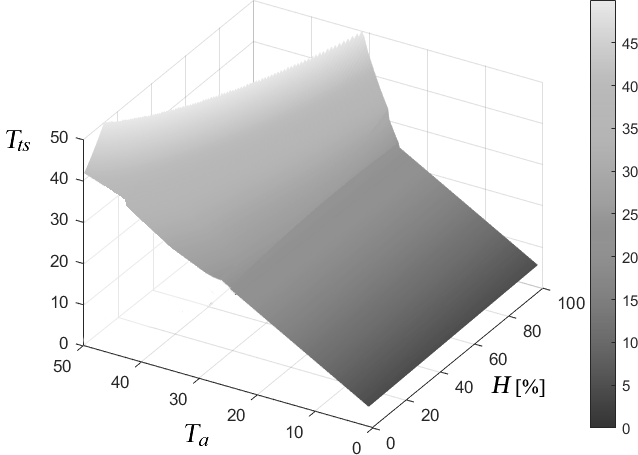
Fig. 20 Variation of the heat index with ambient temperature and humidity
It can be seen that the dependence on humidity is minimal as long as Ta < 25°C, but above this temperature, the contribution to the heat sensation is large.
To include the heat index in the measurement of the percentage of dissatisfied users Disc, it is used instead of the ambient temperature in (7). The result is shown in Figure 21.
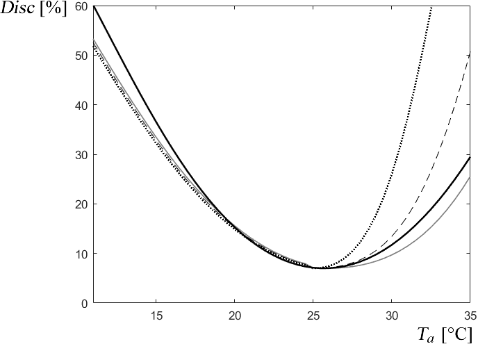
Fig. 21 Disc variation with ambient temperature and various humidity conditions: Grey line: H = 25%; Dashed line: H = 50%; Dotted line: H = 75%; Full black line: without considering humidity
In accordance with Fig. 20, the effect of humidity on the percentage of dissatisfied users is minimal at Ta < 25°C but very noticeable above this temperature.
Figure 22 shows the evolution of the percentage of dissatisfied users Disc, the ambient temperature Ta and the mean radiant temperature Trm, which are responsible for the behaviour of the former, with a variation in the outside temperature Te between 20°C and 35°C, typical of the summer season in the area. The va air speed was 0.2 m/s and the humidity H was around 40%. The HVAC system was not in operation.
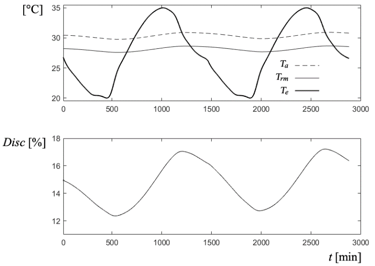
Fig. 22 Evolution of the Disc percentage of dissatisfied users in a 48hs trial
4. RESULTS
The model developed enables tests to be carried out to simulate the process under different conditions. Particularly noteworthy are the variables subject to further optimisation, especially the relative power consumption Pr and the percentage of dissatisfied users Disc.
Figure 23 shows the behaviour of the wall temperature Taa, which follows the setpoint SP over a wide range of temperature references between 15°C and 24°C.
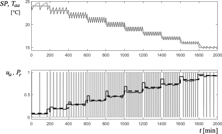
Fig. 23 SP reference variation test over a wide range
In this simulated experiment, the outdoor temperature Te is kept constant to show the almost linear behaviour of the relative power Pr with the setpoint SP.
Two relative powers have been plotted: in the thick grey solid line, the power measured during the period tp, which considers a single ON/OFF cycle of the HVAC compressor. The dashed line shows the relative power calculated over the period when SP was constant. The bottom graph shows the variation of the ratio between the ON and OFF times of the control signal ua (thin line) and the progressive increase of the relative power consumption when SP decreases, as expected. As this test is designed to analyse the behaviour of the relative power consumption, the percentage of dissatisfied users, which increases as the temperature drops below the neutral temperature of 25°C, was not plotted.
Figure 24 illustrates a reverse scenario, where the SP reference of the HVAC remains constant at 23°C, and the response to a conventional outdoor temperature variation Te is observed over 48 hours. The relative power Pr follows a quasi-sinusoidal pattern corresponding to changes in both the ambient temperature Ta and the mean radiant temperature Trm. The same applies to the percentage of dissatisfied users Disc, which remains below 10% and is therefore considered acceptable according to current standards.
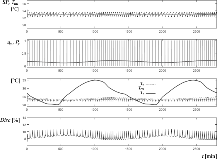
Fig. 24 System evolution with constant SP reference
5. CONCLUSIONS
A dynamic grey box model was developed to predict the temporal evolution of temperatures and humidity in a workspace of the UNSJ Faculty of Engineering. The simulated variables follow the measured variables with sufficient accuracy, which makes this model suitable for MPC control. It does not require detailed knowledge of the physical parameters of the various system components, as is common in a theoretical white box model, nor does it require large data packages that completely cover all operating states of the system, as is the case with data-driven black box models. The internal variables involved allow the prediction of the necessary measures for a subsequent MPC multi-objective supervision of the environment climate: the power consumption of the HVAC and the percentage of dissatisfied users with the thermal environment.
Although previous studies have developed grey box models, this study is original and provides new insights because
It takes into account the internal dependencies between variables.
It includes relative humidity in the model.
It uses LPV versions of some sub-models to allow a better description of the non-linear relationships.
It also considers the effect of forced cross-ventilation from outside, which can help to reduce the power requirements of air-conditioning.
It defines the relative power of an HVAC in the post-occupancy phase and makes it possible to be independent of the absolute power [W] consumed by the equipment. This facilitates the subsequent optimisation process.
The methodology for determining the model parameters is straightforward and easily replicable and can therefore be adapted to determine other environments.
Reducing energy costs without compromising the quality of life in the operation of buildings is a public objective, as it contributes to the cost-effective energy transition. Conserving energy resources and reducing environmental impact is a condition to be achieved through sustainable buildings and cities. Applying this dynamic model to optimise the air conditioning of a building with current equipment would not only extend its lifespan but also avoid the tendency to replace it with more efficient equipment.
6. FORTHCOMING DEVELOPMENTS
Using the developed model, the multi-objective predictive supervision technique will be applied to obtain the air speed profile and HVAC setpoint that will be applied to the system.
A strategy will be designed for online updating of the described model is designed. In this way, seasonal variations will be captured better.
